

Reinforcement learning (RL) has played a crucial role throughout the history of research on large language models (LLMs). Through RL, we created early versions of instruction following models, made important advancements in alignment and safety, and enabled LLMs to solve complex reasoning problems. Despite the many breakthroughs, however, RL remains one of the most rapidly evolving areas in AI research. Many of the most pressing problems we are trying to solve today—reasoning, knowledge work, agents, token efficiency, reliability, and more—are being addressed through RL. In this overview, we will work up to the frontier of RL research by starting from first principles. In a single overview, we will cover the fundamentals of RL, the full evolution of policy gradient algorithms currently used to train LLMs, and several recent areas of emerging research in RL.
Related reading. This overview aims to be a standalone reference that can be used to learn the foundational concepts of RL research. However, most of the content is a synthesis of resources and blogs—both external and written by myself—that have been published over the course of many years. Key information will be provided in each section of the overview. Most sections will end with a link to a more in-depth blog that provides advanced details and research on that topic. Beyond these supplemental blogs linked within each section, numerous external resources have been incredibly helpful in creating this resource:
The RLHF Book by Nathan Lambert.
Reinforcement Learning by Richard S. Sutton and Andrew G. Barto.
Spinning Up in Deep RL from OpenAI.
Build an LLM / Reasoning Model from Scratch by Sebastian Raschka.
Policy Gradient Algorithms by Lilian Weng.
A Vision Researcher’s Guide to RL by Yuge (Jimmy) Shi.
From REINFORCE to Dr. GRPO by Qingfeng Lan.
Async GRPO in the Wild by Yumo Xu.
Open RL infrastructure like TRL and OpenInstruct.
Fundamentals of RL for LLMs
To understand RL for LLMs, we must start by building the necessary background knowledge on general concepts in RL. This section will focus on explaining fundamental concepts upon which the RL algorithms we will see later in the post are based. Specifically, we will provide a formal structure for RL, as well as outline the learning objective used for RL training. Then, we will extend these ideas by covering how RL is formulated in the context of LLM training.
A General Framework for RL
When running RL training, we have an agent that iteratively takes actions within some environment; see below. Each step in this iterative process is denoted with a time step t, and we denote the action at time t as a_t.
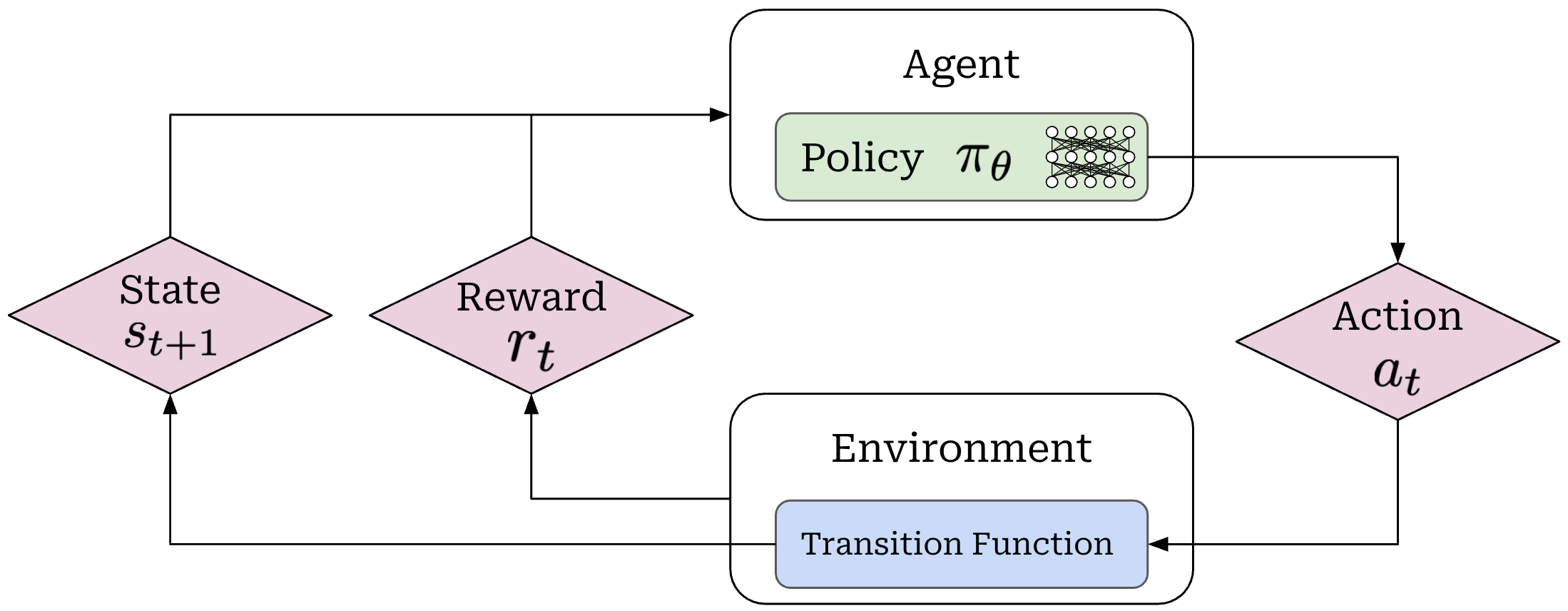
These actions are predicted by a policy—we can think of this as the agent’s brain—with parameters θ (e.g., the policy is the LLM itself in the context of training an LLM). Our policy can either be deterministic or stochastic, but for LLMs we will assume the policy is stochastic. Our stochastic policy π_θ outputs a probability distribution over the set of possible actions, and an action a_t is sampled from this distribution. We denote the probability of an action as π_θ(a_t | s_t).
When the policy outputs an action, the state of the environment will be updated according to a transition function, which is part of the environment. The state at time t is denoted as s_t. Our transition function is written as P(s_t+1 | a_t, s_t). However, we will soon see that transition functions are less relevant in the context of LLMs, though they do still play a role in specific settings (e.g., agents).
After an action is taken, the environment provides a reward, which characterizes the desirability of a given state or action. The reward may be positive, negative, or zero, and the reward granted at time step t is typically denoted as r_t. Intuitively, we can conceptualize RL as a trial and error process. As our agent acts in its environment, the training process reinforces—either positively or negatively—observed behavior via the reward. Hence, the name “reinforcement” learning.
Beginning from an initial state s_0 that is sampled from a distribution d_0 over the set of initial states, the agent will repeatedly:
Sample actions (
a_t).Transition to a new state (
s_t+1).Receive a reward (
r_t).
This process will continue until the final state s_T is reached—either because this is a terminal state or a pre-defined maximum number of steps has been reached. Together, the sequence of steps in this process form a trajectory; see below.

The RL training process repeatedly samples trajectories from the agent in this manner. In this way, the agent is allowed to explore the space of possible states and actions, ultimately discovering behavioral patterns yielding high reward.
The Learning Objective for RL
As discussed before, each step of a trajectory is sampled according to two probability distributions:
The action distribution
π_θ(a_t|s_t)predicted by our policy given the current state at timet.The next state distribution
P(s_t+1|a_t,s_t)given by our transition function for the current states_tand sampled actiona_tat timet.
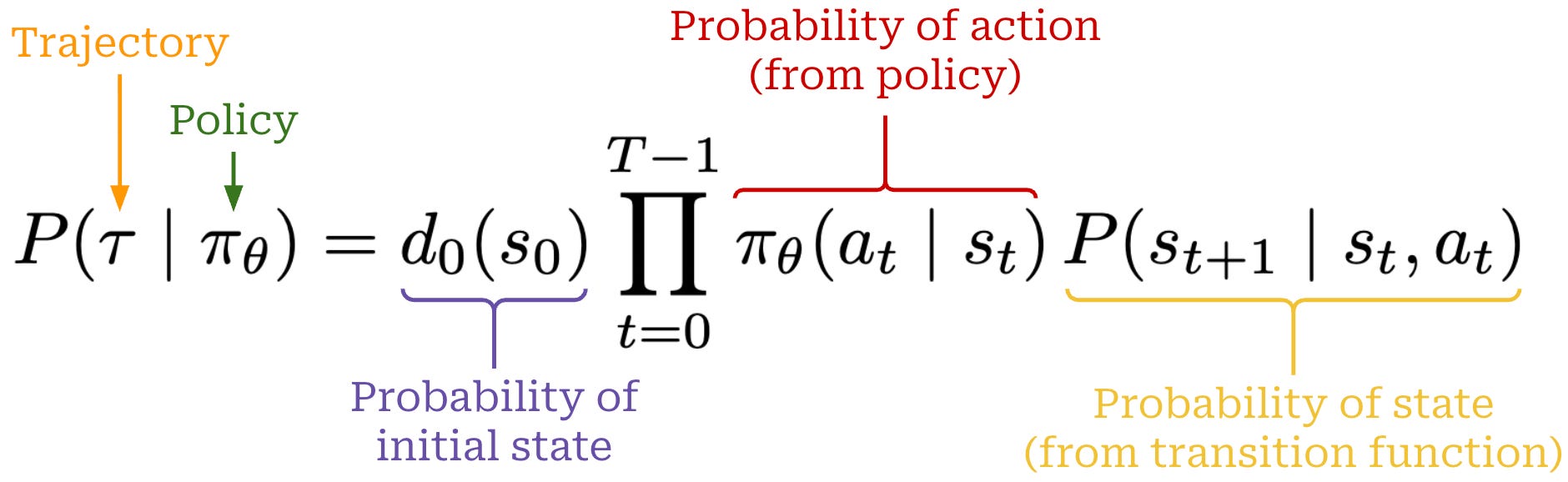
By using the chain rule of probabilities, we can use these two distributions to calculate the probability of an entire trajectory as shown below.
The cumulative reward of a trajectory is simply the sum of r_t values for all time steps t in the trajectory. The cumulative reward is also commonly referred to as the return of a trajectory. There are two common ways to express the return: discounted or non-discounted; see below. The discounted return incorporates a discount factor γ ∈ [0, 1], raised to the power of t, in the sum over rewards. Practically, the discount factor (exponentially) decreases the value of future rewards, encouraging the model to achieve rewards sooner rather than later1.
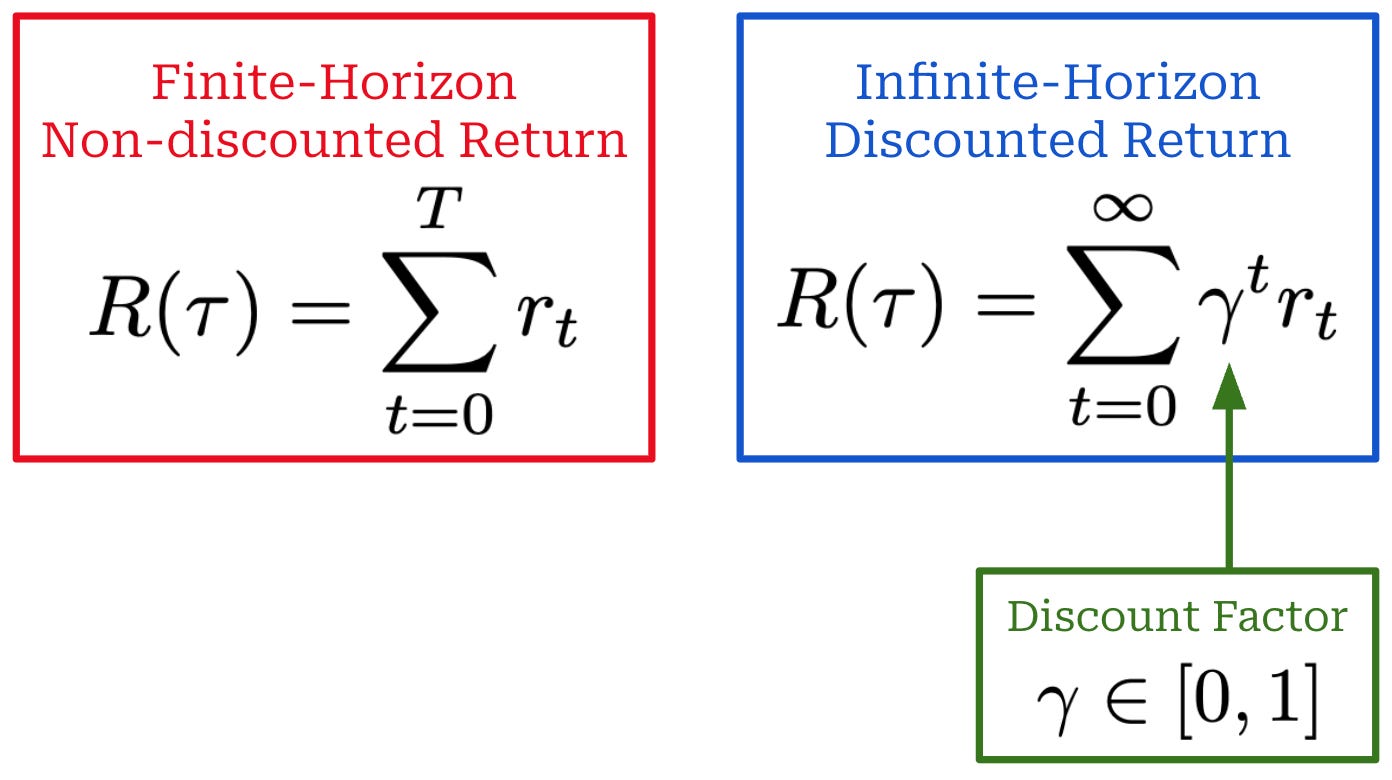
Usually, the non-discounted return is expressed using a finite horizon, meaning that the total length of the trajectory T is finite. In contrast, the discounted return is typically expressed with an infinite horizon (i.e., T = ∞), as shown above. For LLM post-training, we often have a finite T and γ = 1 because we primarily use rewards earned at the trajectory (or completion) level rather than at individual states. As we will see throughout this overview, however, this is not always the case. For example, KL penalties are often formulated as a per-token reward and GAE uses a discount factor when estimating the advantage.
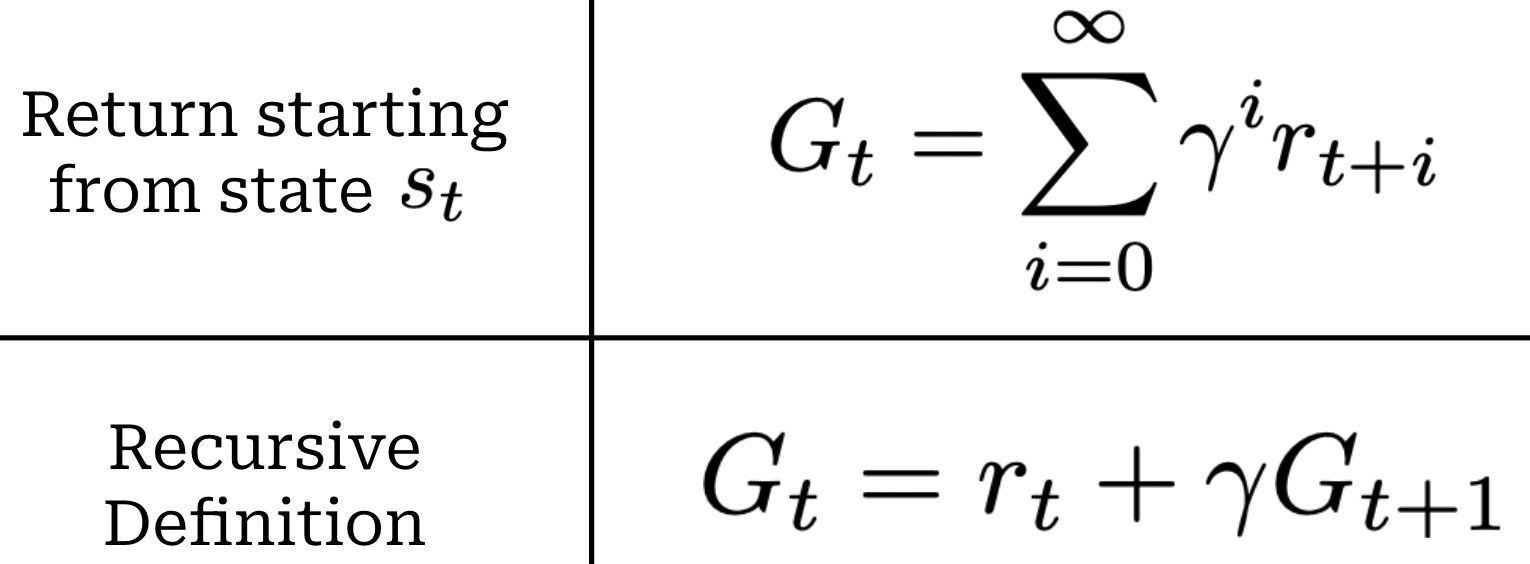
Instead of expressing the return over an entire trajectory R(τ), we can also formulate the return G_t beginning at state s_t; see above. Such notation is common in the literature2 and also allows us to express the return recursively.
The objective function for RL is to maximize the expected return of the current policy. We can directly express this objective as an expectation taken over sampled trajectories, which can be written either as an integral or a discrete probability-weighted sum over possible trajectories; see below.

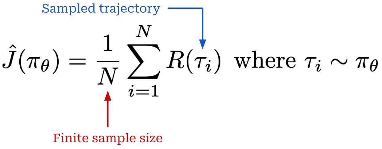
In practice, computing the expected return as a discrete sum over all possible trajectories is not feasible (i.e., there are far too many possible trajectories to enumerate them explicitly). Instead, we take a Monte Carlo estimate3 of this objective using the returns of randomly-sampled trajectories; see below.
Value and advantage functions. The RL objective considers the expected cumulative reward of a policy. Related to this objective, we have the following set of functions (shown below) that are commonly referenced in RL:
Value Function
V(s): the expected cumulative reward when you start in statesand act according to your current policyπ_θ.Action-Value / Q Function
Q(s,a): the expected cumulative reward when you start in states, take actiona, then act according to your policyπ_θ.Advantage Function
A(s,a): the difference between the action-value and value function; i.e.,A(s,a)=Q(s, a)-V(s).
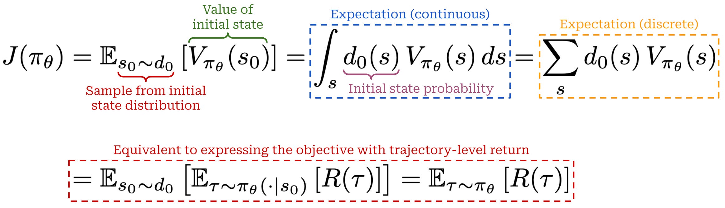
The value function V(s) is highly related to our objective for RL. The value function also considers the expected return, but—unlike the RL objective—it conditions this expectation on the current state s; see below. In contrast, the RL objective takes an expectation across all trajectories that can be generated by the current policy under a given initial state distribution.

We can even formulate our RL objective in terms of the value function as shown in the figure below. This expression is equivalent to the prior trajectory-based return formulation of the RL objective. We are expressing the objective as the expected value starting from a state sampled from our initial state distribution.
The action-value function is similar to the value function in that it conditions upon the state s. However, the action-value function also conditions upon the action a taken in that state. Therefore, both of these functions measure expected return, but the expectation is taken under different conditioning.

The advantage function captures the relative utility of action a. Intuitively, V(s) captures the expected return when acting according to the policy from state s, while Q(s, a) represents the expected return when:
Starting from state
s.Specifically taking action
a.Acting according to our policy afterward.
The difference of these quantities, A(s, a) = Q(s, a) - V(s), measures the difference between the expected return from state s and the expected return from state s specifically after taking action a. By taking this difference, the advantage function intuitively captures how much better or worse the action a is relative to the policy’s expected performance from state s. The advantage is positive when the expected return after taking action a is higher than expected for state s and vice versa. As we will learn, advantage functions play a huge role in RL research.

“Sometimes in RL, we don’t need to describe how good an action is in an absolute sense, but only how much better it is than others on average. That is to say, we want to know the relative advantage of that action. We make this concept precise with the advantage function.” - Spinning up in Deep RL
Value and advantage estimation. We have formulated the value, action-value, and advantage functions above as expectations. However, these expectations cannot usually be computed exactly in practice—we need some way to estimate them. A natural approach is to use information from actual trajectories sampled from the current policy. In particular, the observed return G_t after taking action a_t provides a Monte Carlo estimate of the action-value function Q(s_t, a_t).
Intuitively, G_t captures what actually happened after taking a particular action a_t in state s_t. A single sampled return is a noisy estimate of Q(s_t, a_t). To reduce the variance of this estimate, we can also take an average of the return across multiple samples. On the other hand, the value function V(s_t) captures the expected return from a state s_t before committing to any particular action a_t. When working with policy-gradient methods, there are two approaches that we will encounter for estimating the value function:
We can avoid explicitly estimating the value function and instead estimate the advantage function by subtracting a simple baseline—such as the average return across a batch—from the action-value function.
We can directly approximate the value function using a learned value model, also referred to as a critic.
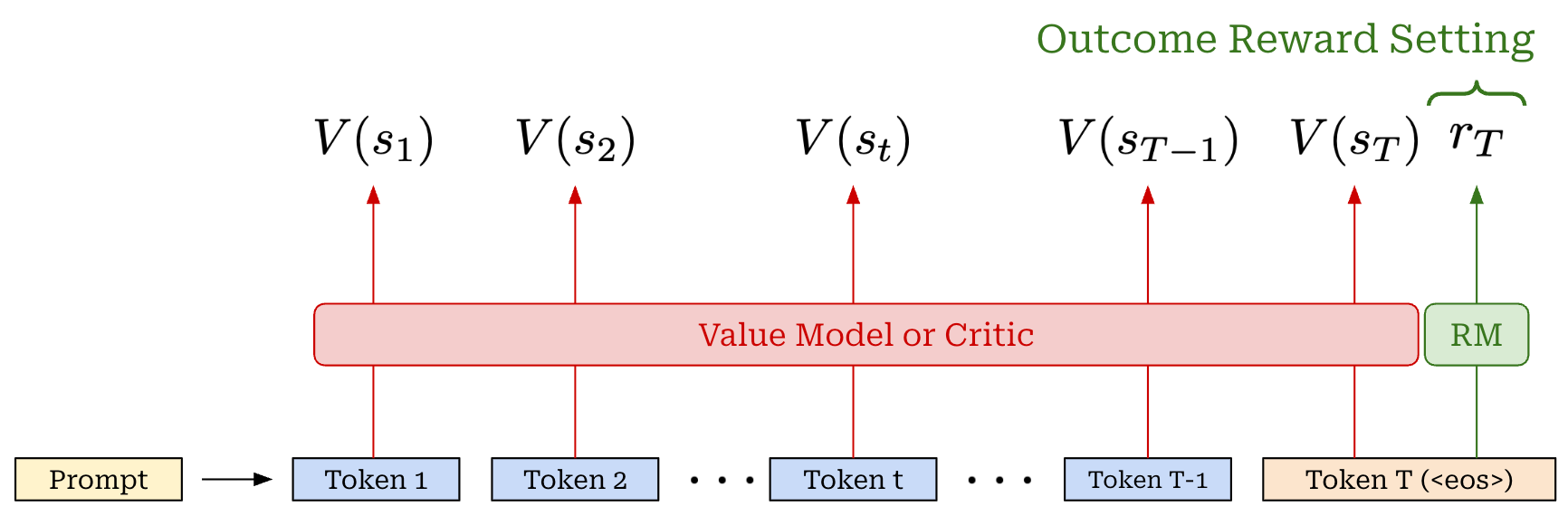
In the LLM domain, a critic is typically implemented using an LLM backbone with an additional scalar value head—this is very similar to the architecture of a reward model. Unlike reward models, however, the critic predicts the expected future return for each token position—or state—within the sequence, rather than a single reward for the entire sequence. Because we are using an LLM with a decoder-only (causal) architecture, the LLM’s representation at each position t only depends upon preceding tokens. Therefore, a single forward pass can predict value estimates for every token within the trajectory; see below. Although we will learn more details later in the post, the critic is trained alongside the policy via a regression loss between its predictions and the actual observed returns.
From here, we can construct a simple estimate of the advantage function; see below. Given that A(s_t, a_t) = Q(s_t, a_t) - V(s_t), we can estimate the advantage by taking the difference between G_t—a sample estimate of Q(s_t, a_t)—and our value model outputs—an approximation of V(s_t).
# B - batch size
# L - sequence length

# sampled return from each state/action
returns = ...                                      # (B, L)

# estimated value of each state
values = critic(states)                            # (B, L)

# compute advantage estimate
advantages = returns - values.detach()             # (B, L)
Intuitively, G_t tells us what actually happened after taking action a_t, while the value model predicts what we expected to happen from state s_t. Therefore, their difference estimates whether the sampled action produced an outcome that was better or worse than expected. As we will see, RL algorithms differ in how they estimate returns, values, and advantages, but these estimates build upon the same underlying quantities defined above.
Optimizing the objective. We want to maximize the RL objective during training—our policy should output trajectories with high returns. Just like any other learning objective, the expected return can be maximized with gradient ascent; see below.

To perform gradient ascent, however, we must be able to compute the gradient of this objective with respect to the parameters of our policy. We call this a policy gradient in RL research, and there are many ways the policy gradient can be estimated. In fact, nearly all of the algorithms we will study in this overview are policy gradient algorithms: they propose some technique for computing the policy gradient then optimize the policy via gradient ascent. In the LLM domain, policy gradient algorithms are by far the most common choice for RL training.
Formulating RL for LLMs
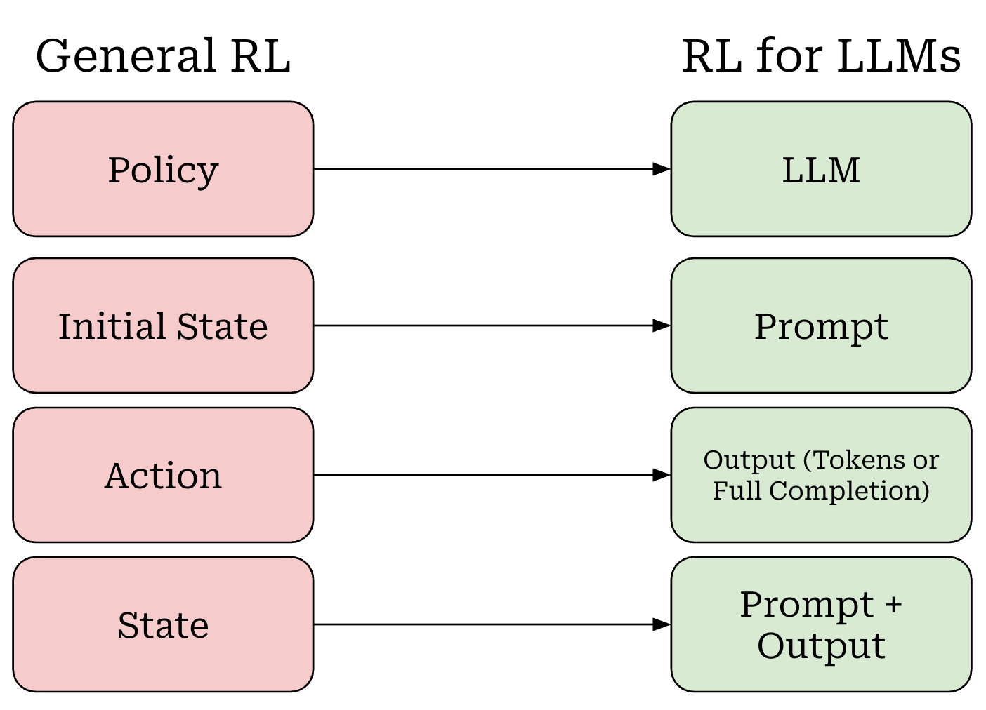
Now that we understand RL basics, we need to map the concepts that we have learned onto LLM training in particular. Even in the LLM domain, RL follows the same basic setup that we saw before. Starting from an initial state, our policy acts in a loop until a terminal state is reached, thus yielding the final trajectory. As shown above, these terms map onto the LLM domain as follows:
Our policy is the LLM itself.
Our initial state is the prompt.
Depending on the formulation, an action can correspond to either a single token or the entire completion.
Our state is the combination of our prompt with tokens generated so far.
The entire completion from the LLM forms a trajectory.
This setup is just next token prediction. Given an initial prompt, our policy—the LLM being trained—takes actions by autoregressively generating tokens in a loop; see below. Eventually, a terminal state is reached (e.g., an end of sequence token), leading the generation process to complete. The trajectory produced by this process includes the prompt along with the full sequence generated by the LLM.
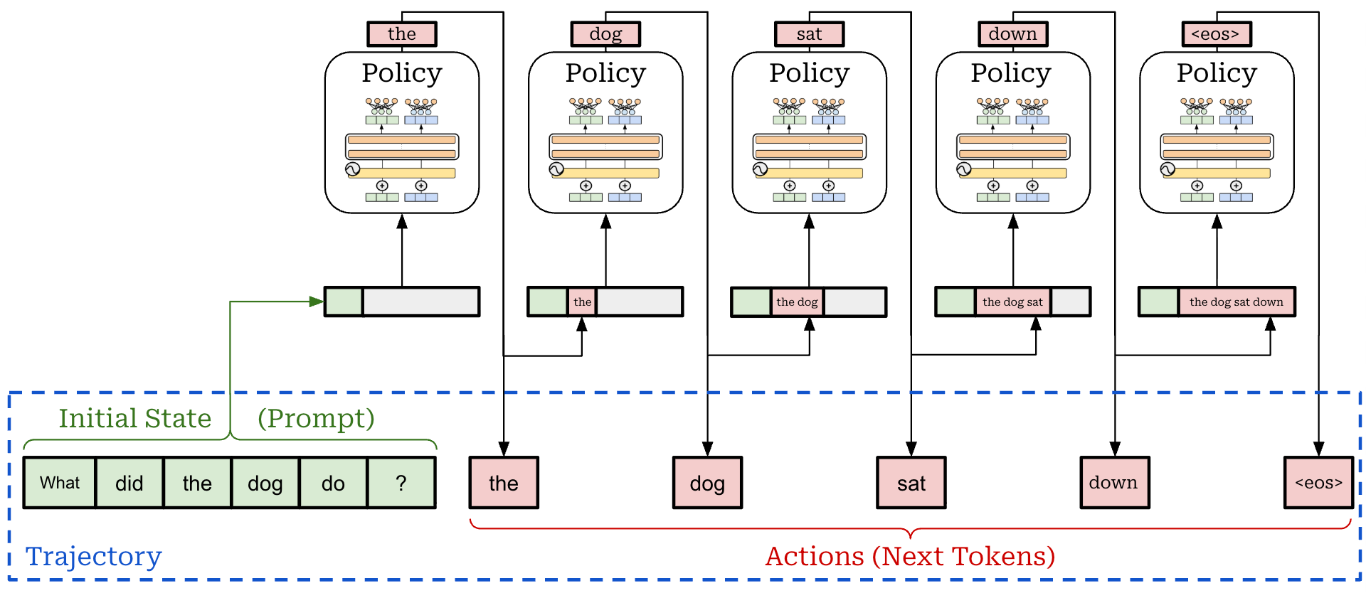
Notably, the transition function in this setup is deterministic. Starting with a prompt x, if our LLM predicts tokens t_1 and t_2 given x as input, our updated state simply becomes s_2 = {x, t_1, t_2}. Our state begins with the prompt x and is updated by concatenating each new token generated by the LLM to the state.
MDP formulation. For LLMs, there are two primary ways in which RL can be formulated that differ in how they model actions. As mentioned above, we can model each token in the next token prediction process as an individual action, which is referred to as a Markov Decision Process (MDP) formulation. An MDP is simply a probabilistic framework for modeling decision-making that includes states, actions, transition probabilities and rewards—this is exactly the setup we have discussed so far for RL! The MDP formulation used for RL is shown below.
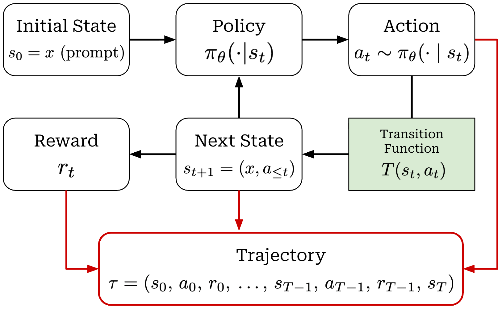
When modeling RL with LLMs as an MDP, our initial state is the prompt and our policy acts by predicting individual tokens. Our LLM is a stochastic policy that predicts a probability distribution over tokens. During generation, an action is taken at each step by selecting a token from this distribution. After a token is predicted, it is added to the state and used by the LLM to predict the next action or token! Eventually, the LLM predicts a stop token (e.g., <|end_of_text|> or <eos>) to complete the generation process, thus yielding a complete trajectory.
Reward granularity. So far, our formulations have depicted a reward r_t being assigned to every step of the generation process4. When training LLMs with RL, however, there are two granularities at which rewards are usually granted for the LLM’s completion:
Outcome rewards are awarded to the entire completion.
Process rewards are granted at intermediate steps in the completion.
These two types of rewards are depicted below. Outcome rewards are the most common in recent LLM training setups, as we can provide a reward based upon the correctness of a completion. However, outcome rewards are sparse—they tell us whether the entire completion is good or bad—which can make learning difficult. In contrast, process rewards can improve learning efficiency by enabling granular credit assignment at several intermediate stages within the full completion.

Bandit formulation. Given that outcome rewards are a common setup for RL with LLMs, we may wonder: Does it really make sense to model each token as its own action? A reward is assigned only after the LLM generates a complete response, meaning that no rewards would be granted on a token level. Instead, we could model the entire response as a single action that receives an outcome reward. This is the key idea behind the bandit formulation for RL training; see below.

This name comes from the idea of a contextual bandit in probability theory. The bandit setup is simple: our agent chooses an action, receives a reward and the episode ends. Our complete trajectory is a single action and reward! For LLMs, our action is the full completion generated for a prompt, which receives an outcome reward. In the bandit formulation, it is also common to use the notation x and y for the prompt and response, respectively (i.e., instead of s and a in the figure above).
“Given that in LLM applications,
r(x, y)is only obtained at the end of the full sequence, it may be more appropriate to model the entire generation as a single action, as opposed to each token.” - from [15]
In the context of LLMs, we already know how to compute the probability of both individual tokens and the full completion for a prompt. Therefore, we have the ability to model RL using either an MDP or bandit formulation. As we will learn, both formulations are commonly used in practice. For example, REINFORCE and RLOO are commonly formulated with a bandit formulation, while algorithms like PPO are typically formulated as an MDP. Both formulations are valid, and we will see several examples of bandit and MDP formulations in this overview.
Computing rewards. There is one final question that we have yet to answer: How do we derive the reward during LLM training? The answer depends on the type of RL training being used. Two broad categories of training are used today:
Reinforcement Learning from Human Feedback (RLHF) trains the LLM using RL with rewards derived from a human preference reward model.
Reinforcement Learning with Verifiable Rewards (RLVR) trains the LLM using RL with rewards derived from rules-based or deterministic verifiers.
These two frameworks are depicted below. In RLHF, we collect a large amount of preference data—composed of a prompt with a chosen and rejected completion—to train a reward model, or an LLM with an added regression head that has been trained to output a preference score given a prompt and completion as input. The reward is directly computed using this reward model during training with RLHF.

In contrast, RLVR derives rewards by checking the correctness of a completion with deterministic verification functions. For example, we can check whether an LLM’s answer to a math question is correct by extracting the generated answer and performing exact string matching—or a symbolic matching approach—against a ground truth. Similarly, we can verify coding tasks by executing a known set of test cases and checking whether an LLM’s generated code passes all of the tests.
“We do not apply neural reward model in developing DeepSeek-R1-Zero, because we find that the neural reward model may suffer from reward hacking in the large-scale RL process, and retraining the reward model needs additional training resources and it complicates the whole training pipeline.” - from [9]
Because RLVR derives rewards from deterministic functions rather than reward models, the risk of reward hacking during training is much lower. For this reason, verifiable rewards enable stable RL training at massive scale, which has led to significant advancements in the capabilities of reasoning models and agents.
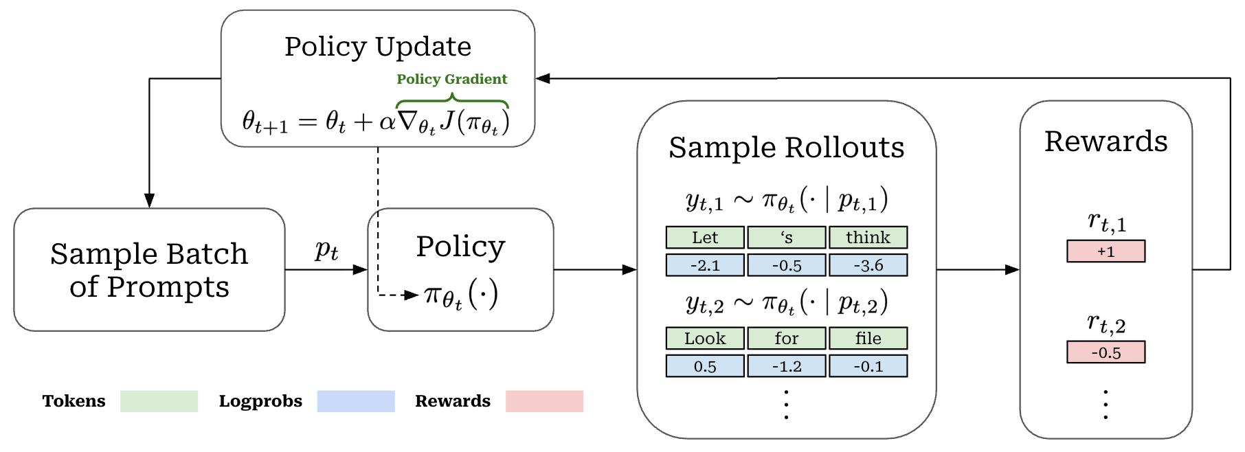
Components of RL training. We will see many variations of RL training in this overview, but they all follow a similar high-level structure; see above. Namely, the RL training process alternates between two key steps:
Rollouts: given a set of prompts, sample completions for each prompt using the current LLM (and compute the reward for each completion).
Policy updates: compute a weight update for the LLM using the sampled rollouts and the given objective function.
The structure of the policy update depends on the RL optimizer being used. In fact, the majority of this overview will focus on outlining the many different algorithms and methods used to handle this policy update!
Kullback-Leibler (KL) Divergence
Throughout LLM post-training, there are many cases where we optimize our model with KL regularization. For example, the canonical optimization objective used within RLHF has the KL regularized form shown below.

As we can see, we want to maximize rewards while minimizing a penalty term—the KL divergence weighted by β—that is subtracted from these rewards. The goal of the penalty term is to discourage our policy from drifting too far away from a reference policy during training. Practically, this KL penalty is incorporated into the RL optimization process in one of two ways:
By directly subtracting the KL penalty from the reward.
By adding a KL penalty into the loss function.
In this overview, we will see the KL divergence incorporated into RL using both of these approaches. For example, initial PPO-based RLHF implementations incorporate KL with respect to the reference policy into the reward, while the original GRPO formulation adds the KL penalty directly into the objective. The exact usage of the KL divergence differs depending on the exact domain. Despite the fact that many forms of regularization exist for LLM training, KL divergence has been a lasting and core component of RL training5. For this reason, we will cover the key details of the KL divergence and how it is used in practice.
KL divergence is a concept from information theory that measures how different a probability distribution is from some reference distribution. The KL divergence is not symmetric—the order of arguments matters. The KL divergence has the form shown below for discrete and continuous probability distributions.

Relation to LLMs. In the LLM domain, KL divergence is commonly used to compare multiple LLMs or policies—usually the policy we are training and a reference policy (e.g., the policy before RL training). Specifically, we compute the KL divergence between the next token probability distributions output by these LLMs. To better understand this, let’s consider a single position t within a sequence. At this position, both LLMs predict a probability distribution over the full vocabulary of possible next tokens. We can then explicitly compute the KL divergence over these two probability distributions as shown below. Notably, this expression is just the discrete formulation for the KL divergence outlined above.
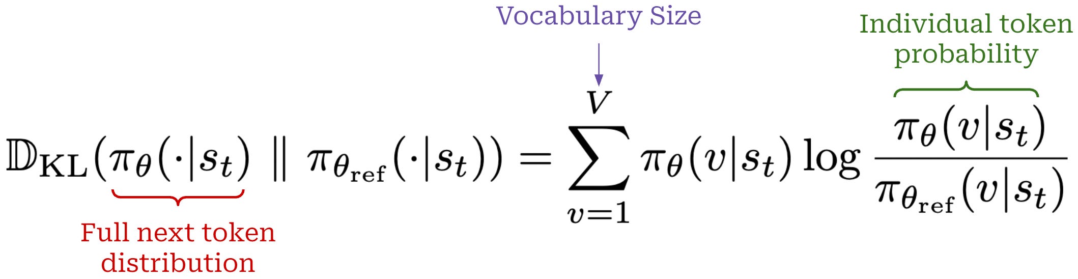
Intuitively, KL divergence measures how much the current policy's distribution over possible next tokens has shifted relative to the reference policy at state s_t. To measure divergence across an entire completion, we can sum KL terms across token positions. More generally, the sequence-level KL is obtained by taking an expectation of these terms over states sampled from the current policy.
Estimating KL divergence in practice. Computing the exact KL divergence requires comparing the full vocabulary distributions produced by the current and reference policies at every token position. Given that we are often working with large vocabularies and long sequences with LLMs, retaining and handling the full token distribution would produce a significant increase in compute and memory overhead. In practice, RL algorithms often use cheaper Monte Carlo estimators of the KL divergence that only require the log probabilities of tokens sampled in the completion—we typically refer to this as a “sampled” estimate of the KL divergence.
Because the KL divergence can be written as an expectation under the current policy, sampling actions from π_θ, computing their log probability ratios, and averaging across samples yields a Monte Carlo estimate of the true KL divergence. We will now cover several options for how the KL divergence can be estimated, and we will adopt the notation from [4] in this discussion.

A simple and commonly-used estimator of the KL divergence is the k_1 estimator; see above. Again, this estimator only considers the probability of the token sampled by the policy a_t, rather than the full vocabulary distribution. In expectation over actions sampled from the current policy, this quantity is equal to the KL divergence. Therefore, the k_1 estimator provides an unbiased Monte Carlo estimate of the true KL divergence, but the variance of this estimate can be high. For example, k_1 can be negative in value, which is not true of the actual KL divergence. A commonly used alternative is the k_3 estimator; see below.
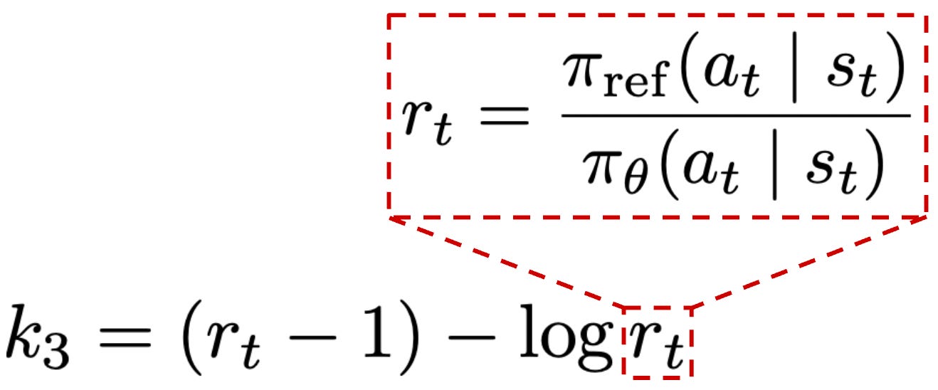
This estimator again only considers the probability of the token actually sampled from the current policy in the completion, rather than the full distribution over the vocabulary. The k_3 estimator matches the KL divergence in expectation, is non-negative for every sampled token, and typically provides a lower-variance estimate relative to k_1. For this reason, the k_3 estimator is an attractive choice for RL training. We will see both of these estimators used in this overview.
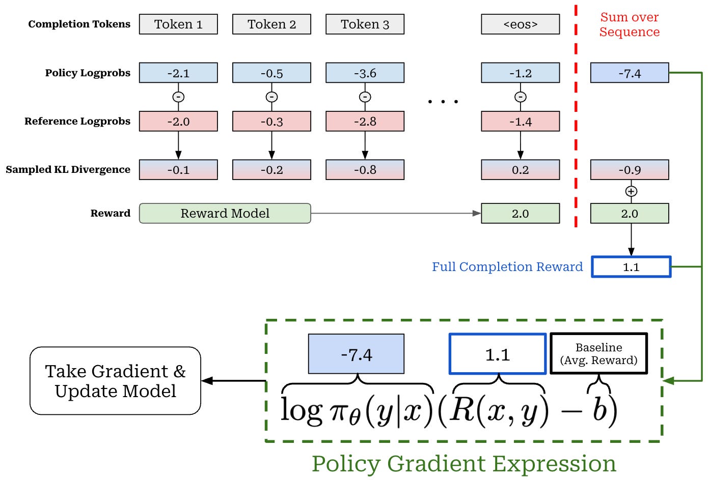
KL implementation. By adopting these estimators, we can approximate the KL divergence for regularization purposes during RL without needing to explicitly sum across the entire vocabulary. Instead, we can sample completions from the current policy, compute current and reference log probabilities of sampled tokens, and estimate the KL divergence using k_1 or k_3; see below.
"""
Assume we already have sampled logprobs.

per_token_logps: logprobs from current policy
reference_per_token_logps: logprobs of sampled tokens under ref policy

B - batch size
L - completion length
"""

# k1 KL estimator
kl_div_k1 = (per_token_logps - reference_per_token_logps)  # (B, L)

# k3 KL estimator
log_ratio = (reference_per_token_logps - per_token_logps)  # (B, L)
kl_div_k3 = (torch.exp(log_ratio) - log_ratio - 1)  # (B, L)

# aggregate across completion tokens
seq_kl_k1 = (kl_div_k1 * completion_mask).sum(dim=-1)  # (B,)
seq_kl_k3 = (kl_div_k3 * completion_mask).sum(dim=-1)  # (B,)
As mentioned before, these per-token KL estimates can be incorporated into the reward or as a penalty into the RL objective function and aggregated across the entire completion or sequence as implemented above and depicted below.
Importance Sampling
In RL, the policy used to generate rollouts does not always perfectly match the current policy we are optimizing. For example, algorithms like PPO may perform multiple policy updates over the same rollouts, while recent asynchronous RL infrastructure may lead to the incorporation of mildly stale or off-policy data into the training process. Importance sampling is a general technique in probability theory that can help to correct mismatches of this kind. Formally, importance sampling allows us to estimate an expectation under a target distribution f(x) using samples drawn from a different proposal distribution g(x); see below.
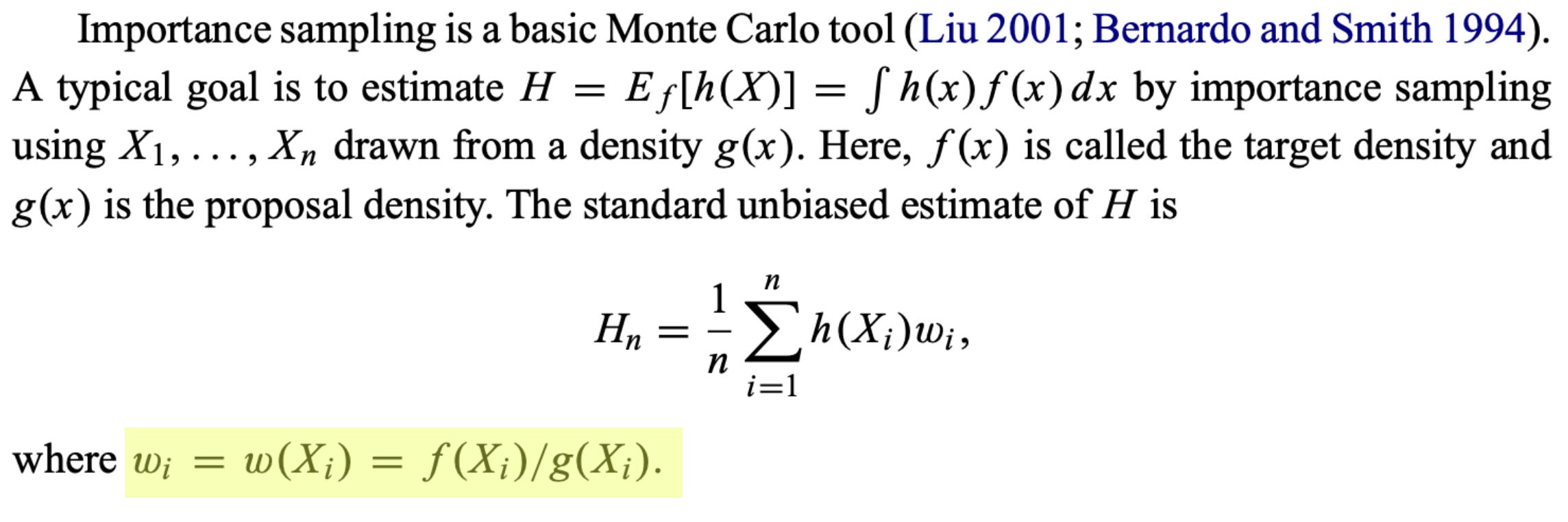
Instead of sampling directly from f(x), we can sample from g(x) and correct for the discrepancy between these distributions using the importance ratio f(x) / g(x). Intuitively, samples that are more likely under f(x) than g(x) receive a larger importance ratio, while samples that are less likely receive a smaller ratio.
Importance ratios appear constantly in research on RL for LLMs. For example, PPO uses an importance ratio to compare the probability of a sampled token under the current policy and the policy that sampled the rollout—this ratio is a core component of the PPO loss function. Additionally, if rollouts are generated using a policy that is different than the policy being optimized—or a separate inference engine that produces slightly different token distributions—we can use importance ratios to account for this mismatch.
In practice, the importance ratio can become large when the distributions differ substantially, yielding unstable and high-variance estimates. For this reason, RL algorithms may choose to clip or truncate the importance ratio, which introduces bias in order to reduce variance and improve stability. We will see examples of both standard and truncated importance sampling throughout the overview.
Policy Gradient Algorithms
In RL, we update our policy such that higher probability is assigned to actions that produce better outcomes. In the LLM domain, our policy is a differentiable neural network, making policy gradient algorithms a natural fit for accomplishing this goal. We can compute the policy gradient with respect to the parameters of our LLM and optimize our policy with gradient ascent. Policy gradient algorithms are by far the most widely-used family of methods for RL training with LLMs.
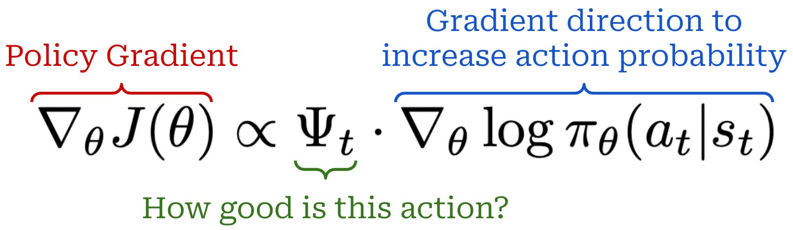
As we might infer from their name, policy gradient algorithms focus on computing the gradient of the RL objective outlined above with respect to the parameters of our policy—the policy gradient. As explained perfectly in the RLHF book, this gradient takes the form shown above and has two key parts:
The gradient of the log probability for action
a_twith respect to our policy parametersθtells us the direction in parameter space that will increase the likelihood of actiona_t.The scalar
ψ_tis a per-action score that allows us to control both the magnitude and direction of this gradient—and the policy update—based on the quality of that action.
For example, actions that lead to bad outcomes can be assigned a large negative value of ψ_t, leading the probability of that action to be decreased significantly and vice versa. Additionally, actions with neutral outcomes can receive a value of ψ_t that is near zero and, in turn, produce very small updates to the policy.
“Some things are simple, such as that
ψ_t>0updates parameters to makea_tmore likely,ψ_t<0updates them to make it less likely. The policy gradient is computing which parameters contribute to an action and if we should make it more or less likely to occur in the future.” - RLHF book
We will now take a look at several of the most popular policy gradient algorithms that are used to train LLMs. These algorithms all build upon the same high-level structure outlined above, but they differ in the approach used to calculate ψ_t and propose various mechanisms to constrain or stabilize policy updates.
Vanilla Policy Gradient (VPG)
As mentioned before, the policy gradient computes the gradient of the learning objective for RL with respect to the parameters of our policy. To derive a simple policy gradient expression, we can use the RL objective defined before—expected cumulative return across trajectories—and take the gradient as shown below.
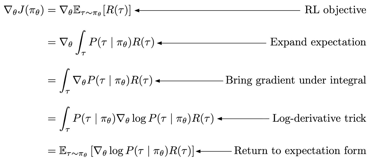
This policy gradient derivation relies on two primary identities:
The continuous definition of an expectation.
The log-derivative trick:
∇_θp_θ(x)=p_θ(x)·∇_θlogp_θ(x).
We can then insert our definition for the probability of a trajectory into the final step of the above derivation; see below. The final result of this derivation is our expression for the Vanilla Policy Gradient (VPG). As we will see, this structure—a sum over action-level log-probability gradients weighted by a return or advantage signal—appears in almost every policy gradient algorithm we will study in this post.
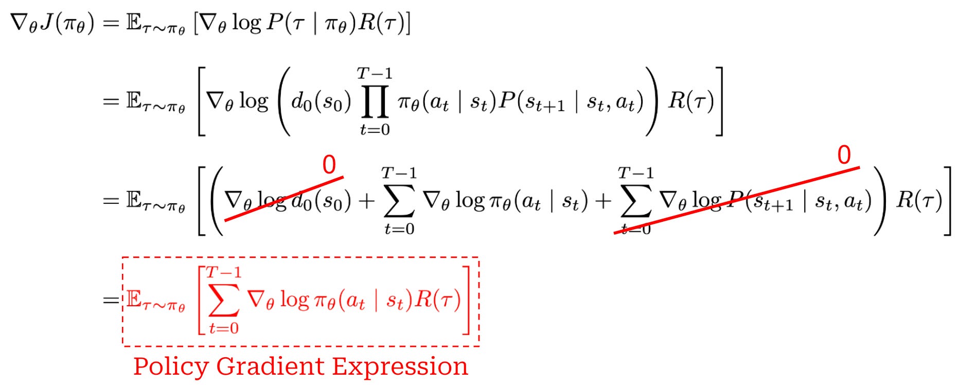
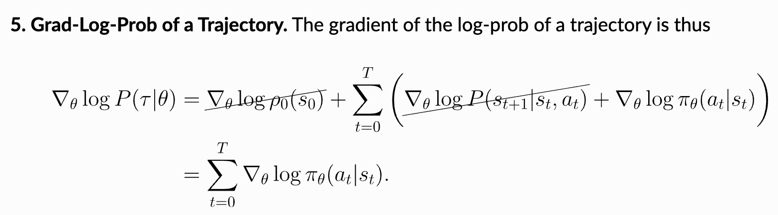
The most complicated part of this derivation is the last step, which transforms the gradient of the log probability of a trajectory into a sum over the gradients of log probabilities of actions. This step does the following:
Inserts our prior expression for the probability of a trajectory.
Converts the product of probabilities into a sum of log probabilities.
Observes that the gradients of the initial state probability and transition function with respect to the policy parameters are always zero (i.e., neither of these components depend on the policy).
VPG implementation. The VPG expression derived above is actually relatively easy to compute in practice, as shown in the implementation below. We adopt a completion-level (bandit) formulation where the entire completion is treated as an action that receives a single outcome reward. As shown before, we can compute the probability of the full completion by summing over the log probabilities assigned to each token. We can then multiply this sequence-level log probability by the completion-level return to compute the VPG loss. In other words, this implementation contains two key quantities:
Completion-level return: a scalar reward assigned to the full completion.
Completion log probability: computed by summing the log probabilities assigned to each token in the completion.
import torch

# B - batch size
# L - sequence length
# V - vocabulary size

# sample completions
# compute (trajectory-level) rewards
with torch.no_grad():
    completions = policy.generate(prompts)
    rewards = reward_model(prompts, completions) # (B,)

# input_ids contains prompt + completion tokens
input_ids = torch.cat([prompts, completions], dim=-1)  # (B, L)

# policy forward pass
logits = policy(input_ids)                       # (B, L, V)

# causal shift (i.e., logits at t predict token at t+1)
logits = logits[:, :-1, :]                       # (B, L-1, V)
sampled_ids = input_ids[:, 1:]                   # (B, L-1)

# get log probs of actions taken by the policy
per_token_logps = torch.log_softmax(logits, dim=-1)
per_token_logps = per_token_logps.gather(
    dim=-1,
    index=sampled_ids.unsqueeze(-1)
).squeeze(-1)                                    # (B, L-1)

# sum log probabilities across actions in each trajectory
# completion mask: (B, L-1), masks out prompt and padding tokens
seq_log_probs = (
    per_token_logps * completion_mask
).sum(dim=-1)                                    # (B,)

# make objective negative because PyTorch minimizes the loss
loss = -(seq_log_probs * rewards).mean()         # scalar

# run single policy gradient update
optimizer.zero_grad()
loss.backward()
optimizer.step()
One key detail that we should notice in the above implementation is that we do not compute the policy gradient directly. Rather, we formulate a loss function for which the negative gradient is equal to the policy gradient then use autodiff in PyTorch to compute the policy gradient—this happens during loss.backward(). The exact loss function used to compute the policy gradient is shown below. This detail is important to understand, as several policy gradient algorithms (e.g., PPO and GRPO) are formulated as a loss function instead of a gradient expression.
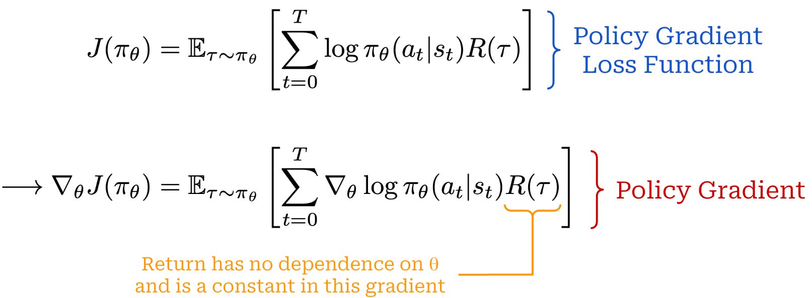
The core intuition behind the structure of the VPG is that we are increasing the probability of actions from trajectories with high rewards. Although this form of the policy gradient is simple, the core expression appears repeatedly and forms the basis for many of the other policy gradient algorithms we will see in this post.
“Taking a step with this gradient pushes up the log-probabilities of each action in proportion to
R(𝜏), the sum of all rewards ever obtained.” - Spinning up in Deep RL
Reducing variance. Despite its simplicity, the VPG expression outlined above suffers from a few notable issues:
The gradients can have high variance because we are estimating the return
G_tfrom a (relatively) small set of rollouts.There is no protection against large, unstable policy updates.
Most policy gradient algorithms aim to solve these problems by reducing the variance of the policy gradient or enforcing a trust region on policy updates (i.e., restricting how much the model can be changed in a single update). By adopting the more generic notation shown below, we can express different variants of the policy gradient algorithm that share a similar structure to the VPG.
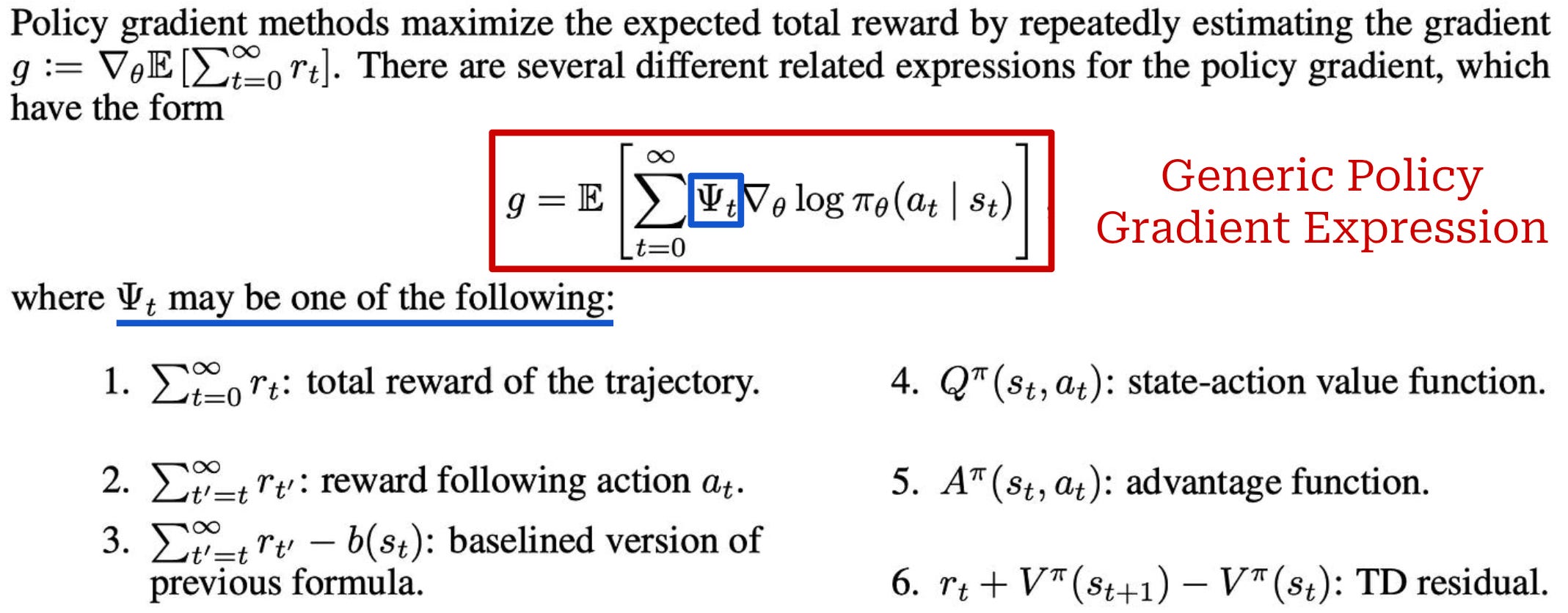
As we can see, this expression is nearly identical to what we saw before. The only difference is that we have switched R(𝜏) with the Ψ_t term, which is a generic term that can represent several possible quantities. For example, we can:
Set
Ψ_t = R(𝜏)to recover our basic policy gradient expression.Set
Ψ_tequal to rewards received after timet(i.e., the reward-to-go policy gradient) to avoid crediting actions with rewards that came before them.Set
Ψ_tto a baselined version of the reward.Set
Ψ_tequal to the state-action or advantage function.
A common theme among these algorithms is the use of baselines, or extra terms—which must not be dependent upon the action a_t—that are subtracted from the reward; see below for an example. Baselines help to center the reward (or value) for a state and can be shown to reduce the variance of policy gradients6. A common choice of baseline is the standard state-dependent baseline b(s_t).
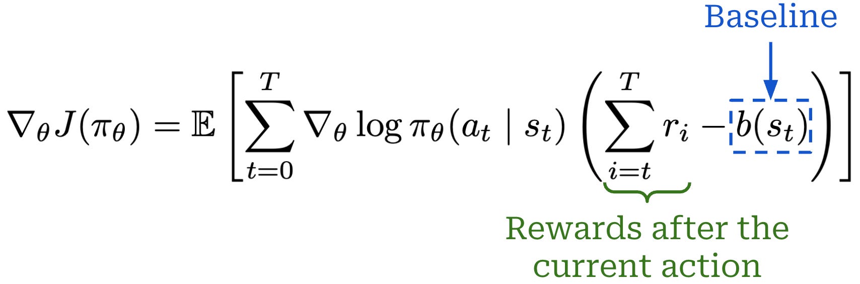
“A common problem with vanilla policy gradient algorithms is the high variance in gradient updates… In order to alleviate this, various techniques are used to normalize the value estimation, called baselines. Baselines accomplish this in multiple ways, effectively normalizing by the value of the state relative to the downstream action (e.g. in the case of Advantage, which is the difference between the Q value and the value). The simplest baselines are averages over the batch of rewards or a moving average.” - RLHF book
This connects directly to our prior discussion of value and advantage estimation. Recall that the sampled return G_t provides a Monte Carlo estimate of the action-value function Q(s_t, a_t). We can choose the value function V(s_t) as our baseline. Because G_t provides a sampled estimate of Q(s_t, a_t), subtracting an estimate of V(s_t) gives us an advantage estimate. Most algorithms set Ψ_t equal to the advantage function, which has a natural credit-assignment signal and substantially reduces the variance of the policy-gradient estimator; see below.
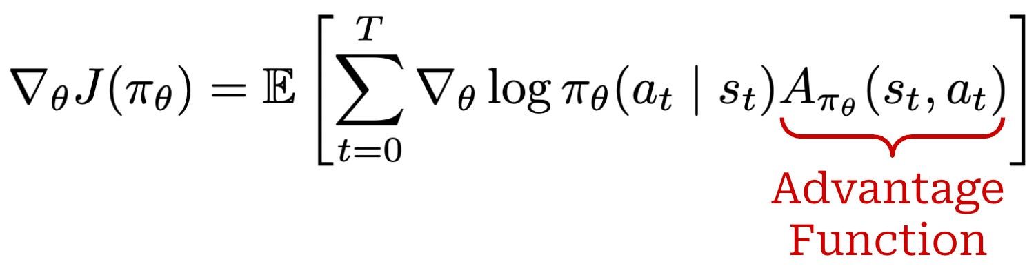
We can estimate the value function with a critic. However, REINFORCE—one of the most popular instantiations of the VPG that we will learn about next—adopts a less expensive approach that leverages simpler baselines.
Further reading. For a full overview of the VPG, how it is derived, and the many variants that exist, please see the deep dive on this topic linked below.

REINFORCE
One of the simplest policy gradient algorithms that can be used for online RL training is REward Increment = Nonnegative Factor x Offset Reinforcement x Characteristic Eligibility (REINFORCE) [3]. VPG provides a basic structure for computing the policy gradient. To compute this gradient in practice, however, we must estimate the expectation in the VPG by sampling trajectories from our current policy. REINFORCE does exactly this—it is a concrete Monte Carlo implementation of the VPG. Recall from the prior section that the VPG is written as an expectation over trajectories sampled from the current policy. REINFORCE simply approximates this expectation using a finite batch of sampled trajectories, making it a direct Monte Carlo estimator of the policy gradient; see below.
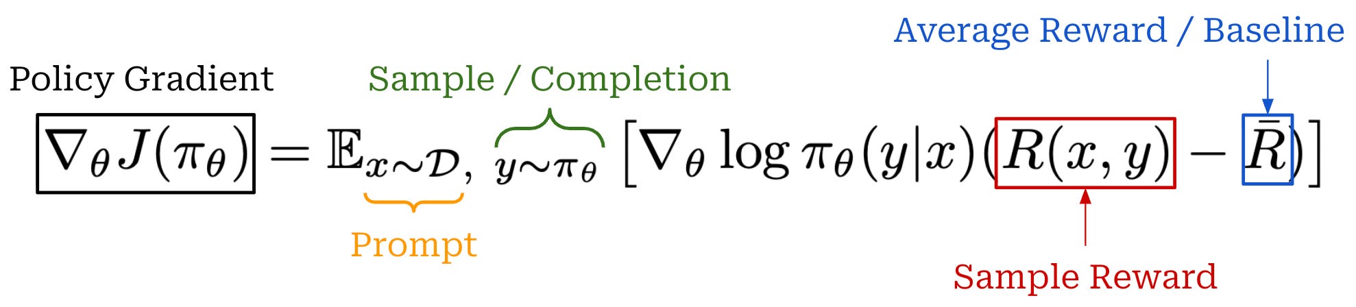
There are several possible instantiations of REINFORCE (we will learn about a few more below) that appear in practice, but we commonly see REINFORCE implemented in a way that matches the baselined VPG. Similar to VPG, REINFORCE can suffer from high variance in its policy gradient—thus leading to training instability or inefficiency—because it forms a Monte Carlo estimate from a finite number of completions. As we already know, we can incorporate a lightweight baseline into this estimate in order to reduce the variance. Any action-independent quantity can be used as a baseline, but a common lightweight choice of baseline for REINFORCE is an average over observed rewards7, such as a batch average or even a moving average throughout training.
Notably, REINFORCE is a strictly on-policy algorithm—we sample completions from the same policy being optimized. Therefore, we do not require an importance sampling correction within the policy gradient expression, as the rollout policy is identical to the policy being optimized. We will see in future sections that this is not always the case. For example, PPO leverages an importance ratio because it can perform multiple policy updates over each set of sampled rollouts, meaning that the data used to update our policy is mildly stale in some cases.
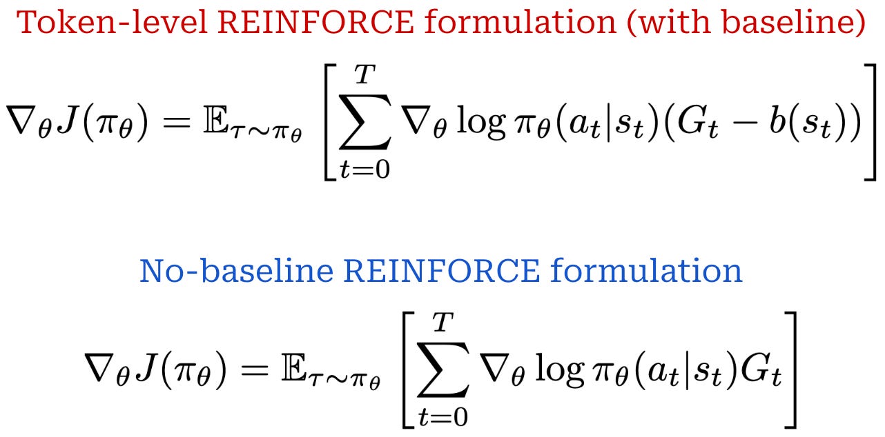
Bandit formulation. The policy gradient expression shown above is formulated at the completion level rather than at the token level. In other words, we consider the entire completion from the LLM to be a single action. Bandit formulations are a common choice for REINFORCE, but we can also adopt a token-level objective as shown below. The key distinction between these formulations is how credit is assigned: a completion-level formulation applies a single sequence-level return or advantage to all tokens, whereas a token-level formulation computes a potentially different return or advantage for each token. Going further, REINFORCE is also commonly formulated without any baseline—this variant is also shown below, where the return is directly inserted into the policy gradient expression.
Key benefits of REINFORCE. Relative to other policy gradient algorithms, REINFORCE is simple and efficient. The policy gradient in REINFORCE can be computed with a single rollout per prompt. During the training process, only the policy is being trained, while the frozen reference policy and—when applicable—reward model are used for inference. In contrast, actor-critic methods like PPO also train a value function, which requires storing another trainable copy of the model in memory and, in turn, increases memory and compute overhead.

What does the acronym mean? The REINFORCE acronym is composed of four key components:
Reward Increment.
Non-negative factor.
Offset reinforcement.
Characteristic eligibility.
The first component is simply our update—or increment—to the policy’s parameters (i.e, using the policy gradient), which is a product of the three other components. The manner in which these components are combined to form the policy update is shown below (top term). To clarify the meaning of each term, we also map the components of REINFORCE to a more familiar policy gradient expression (bottom term). As we can see, this expression is composed of the same terms we have learned about before (i.e., log probabilities, reward, and baseline)!
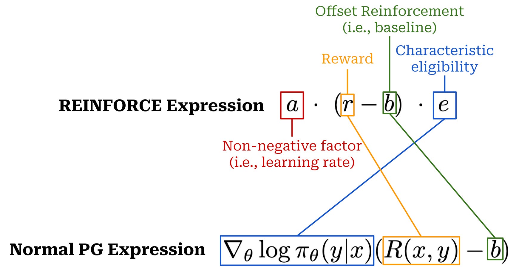
First, REINFORCE includes the learning rate—or a non-negative factor—in its expression for the policy update. The term “offset reinforcement” is also straightforward to understand. The baseline is directly subtracted from the reward in our policy gradient expression. In other words, the baseline is used to offset the reward, which becomes the reinforcement signal in RL (i.e., the reward determines whether actions are good or bad). The baseline is, therefore, an offset to the reinforcement signal. Finally, “eligibility” is a jargon term in RL related to the credit assignment problem—or the problem of determining which specific actions contributed to the reward received by the policy. In REINFORCE, credit assignment is handled by the gradient of the log probabilities of actions under the policy.
“Characteristic Eligibility: This is how the learning becomes attributed per token. It can be a general value, per parameter, but is often log probabilities of the policy in modern equations.” - RLHF book
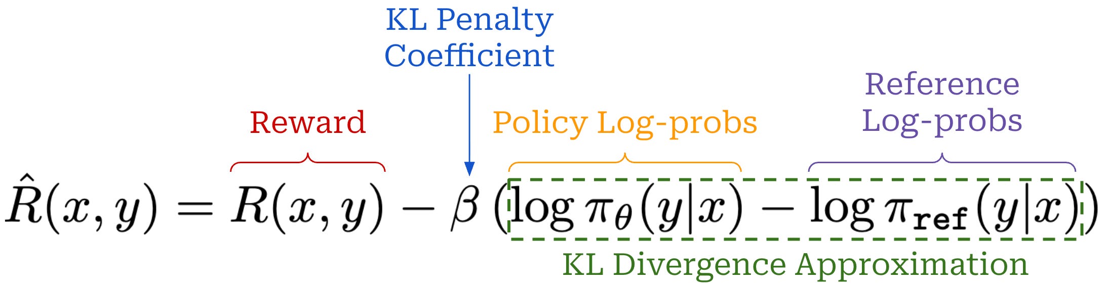
Incorporating KL divergence. When working with LLMs, many implementations of REINFORCE apply a KL penalty between the current policy and a reference policy—usually the initial model checkpoint before RL training—during training. In the figure below, we use the k_1 estimate of the KL divergence between the current and reference policies. For each token in the sequence, this quantity—which considers only the token present in the completion—is a k_1 estimate of the KL divergence between the current and reference next-token distributions. In contrast, the exact KL divergence would compare distributions over the full vocabulary of tokens. We can obtain a sequence-level KL penalty by summing these token-level, sampled estimates across tokens in the completion.
REINFORCE implementation. To make our discussion of REINFORCE more concrete, an implementation of the algorithm in PyTorch is provided below. We should notice in this implementation that policy log probabilities are detached when computing the KL-adjusted reward, which is necessary because the KL is added directly to the reward instead of into the loss function. For this reason, we must treat the reward as a fixed constant when computing the policy gradient.
import torch

# B - batch size
# L - sequence length
# V - vocabulary size

# scaling factor for KL penalty
kl_beta = 0.1

# sample completions
# compute (trajectory-level) rewards
with torch.no_grad():
    completions = policy.generate(prompts)
    rewards = reward_model(prompts, completions) # (B,)

# input_ids contains prompt + completion tokens
input_ids = torch.cat([prompts, completions], dim=-1)  # (B, L)

# policy forward pass
logits = policy(input_ids)                       # (B, L, V)

# causal shift (i.e., logits at t predict token at t+1)
logits = logits[:, :-1, :]                       # (B, L-1, V)
sampled_ids = input_ids[:, 1:]                   # (B, L-1)

# get log probs of actions taken by the policy
per_token_logps = torch.log_softmax(logits, dim=-1)
per_token_logps = per_token_logps.gather(
    dim=-1,
    index=sampled_ids.unsqueeze(-1)
).squeeze(-1)                                    # (B, L-1)

# get log probs of the same actions under the reference policy
with torch.no_grad():
    reference_logits = reference_policy(input_ids)
    reference_logits = reference_logits[:, :-1, :]

    reference_per_token_logps = torch.log_softmax(
        reference_logits, dim=-1
    )
    reference_per_token_logps = reference_per_token_logps.gather(
        dim=-1,
        index=sampled_ids.unsqueeze(-1)
    ).squeeze(-1)                                # (B, L-1)

# compute sampled KL penalty for each action
per_token_kl = (
    per_token_logps.detach() - reference_per_token_logps
) * completion_mask                             # (B, L-1)

# compute return for each trajectory
# outcome reward + sum of token-level KL penalties
returns = rewards - kl_beta * per_token_kl.sum(dim=-1)  # (B,)

# compute baseline and advantage
baseline = returns.mean()
advantages = returns - baseline                  # (B,)

# sum log probabilities across actions in each trajectory
seq_log_probs = (
    per_token_logps * completion_mask
).sum(dim=-1)                                    # (B,)

# REINFORCE loss
# negative because PyTorch minimizes the loss
loss = -(seq_log_probs * advantages.detach()).mean()  # scalar

# run single policy gradient update
optimizer.zero_grad()
loss.backward()
optimizer.step()
This implementation adopts a completion-level (bandit) formulation. Relative to a token-level formulation, the key distinguishing factor is that the full completion is assigned a single scalar return, rather than each token receiving its own return or advantage. More specifically, the KL penalty is initially computed on a per-token basis. However, these per-token KL penalties are summed across the sequence and subtracted from the outcome reward, producing a single (KL-adjusted) return for the entire completion. A completion-level baseline is then subtracted from this return to produce a single advantage, which is applied to the log probabilities of all tokens in the completion.
A corresponding token-level (MDP) formulation would instead retain the per-token rewards, compute a separate return or advantage for each token, and multiply each token's log probability by its corresponding token-level advantage; see below. Notably, such a token-level formulation also naturally supports process rewards. In the code example below, most token-level rewards only include the KL penalty, and an outcome reward is added only to the final completion token. If token-level process rewards are available, however, we can just add these rewards at the corresponding token position before computing the reward-to-go. The return for each token will then capture future process rewards, the outcome reward, and the KL penalties that are already assigned to each token.
# compute per-token rewards
# NOTE: this is just the sampled KL penalty for most tokens
# because we are using an outcome-reward setting
per_token_kl = (
    per_token_logps - reference_per_token_logps
) * completion_mask
per_token_rewards = -kl_beta * per_token_kl.detach()

# add outcome reward to final completion token
positions = torch.arange(
    completion_mask.size(1),
    device=completion_mask.device
)
last_token_idx = (completion_mask * positions).argmax(dim=-1)

per_token_rewards[
    torch.arange(per_token_rewards.size(0)),
    last_token_idx
] += rewards

# compute reward-to-go for each token
returns = torch.flip(
    torch.cumsum(
        torch.flip(per_token_rewards, dims=[-1]),
        dim=-1,
    ),
    dims=[-1],
)

# token-level policy gradient loss
loss = -(
    per_token_logps
    * returns.detach()
    * completion_mask
).sum(dim=-1).mean()
REINFORCE variants. Several variants of REINFORCE modify how the baseline or advantage is estimated while retaining the same basic structure. A prominent example is REINFORCE Leave-One-Out (RLOO), which improves upon the simple batch-average baseline used in our REINFORCE example. Rather than using a global baseline across prompts, RLOO samples K completions per prompt and constructs a prompt-specific baseline from the other K - 1 completions. In particular, the baseline for a completion is the average return of the other K - 1 completions for the same prompt, excluding the completion itself; see below.
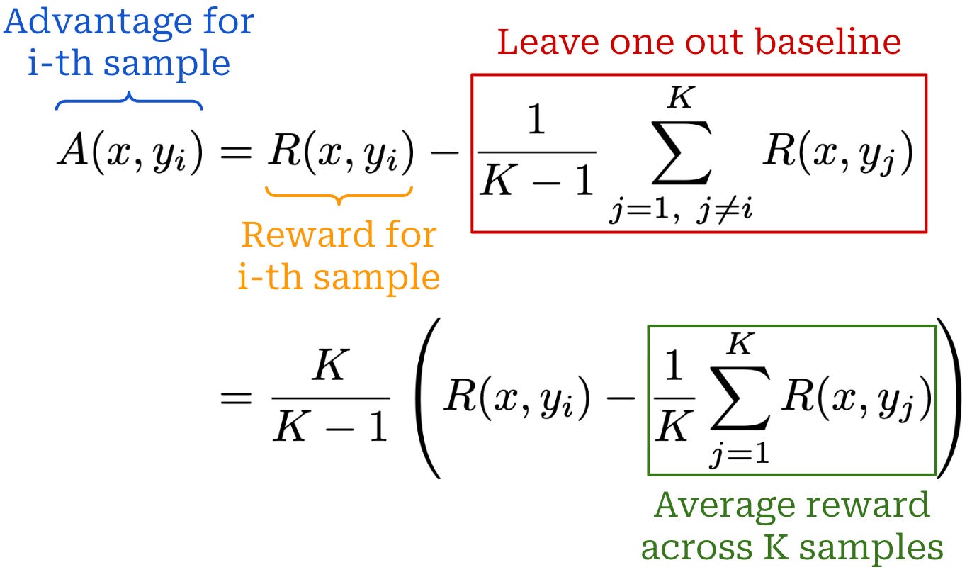
The leave-one-out construction is important because a completion’s own return is not included in its baseline. As a result, the baseline is action-independent, thus preserving the unbiased REINFORCE policy-gradient estimator while providing a stronger (prompt-specific) signal to further reduce variance.
RLOO uses a prompt-specific advantage that measures whether a completion performed better or worse than the policy’s other sampled completions for that prompt. As we will see later, this approach is similar to GRPO-style advantage estimation, and we can even show that RLOO is equivalent—up to a constant scaling factor—to certain GRPO variants. RLOO matches the simplicity of REINFORCE but trades additional inference compute (i.e., we must sample K completions for every prompt) for a better and more stable baseline estimate.
There are also several other REINFORCE variants commonly used in practice. For example, REINFORCE++ combines REINFORCE-style advantage estimation with global advantage normalization and a PPO-style clipped objective.
Further reading. For a deep dive on REINFORCE, including algorithm variants and handling large-scale RL training with LLMs, see the writeup below.

Proximal Policy Optimization (PPO) [6]
From REINFORCE, we learned that the variance of the policy gradient can be reduced by subtracting a simple baseline—the average reward—from the sampled return. However, the Monte Carlo approach used to estimate the policy gradient in REINFORCE, despite being simple and practical, can cause training instability due to high variance policy gradient estimates. To further reduce variance, we can consider a more informative choice for the baseline: the value function V(s_t). As we learned before, the value function—because it is action-agnostic—is a valid baseline that measures the expected return G_t given a current state s_t. If we subtract this value function from the observed return, we are actually forming an estimate of the advantage function: A(s_t, a_t) = G_t - V(s_t).
Actor-critic framework. Using an estimate of the advantage function as a learning signal provides one of the lowest-variance estimates of the policy gradient. Specifically, recall that G_t provides a sampled estimate of Q(s_t, a_t). If we can estimate the value function V(s_t), then we can construct the advantage estimate as G_t - V(s_t), but the value function is unknown.
In REINFORCE, we avoided explicitly estimating the value function and instead used a lightweight, critic-free baseline to compute the policy gradient. However, this approach can lead to high variance. This problem naturally motivates the use of an actor-critic framework, where we simultaneously train both the policy—or actor—and a value model—or critic—during RL. The critic can then be used to obtain a lower-variance advantage estimate relative to a Monte Carlo approach.
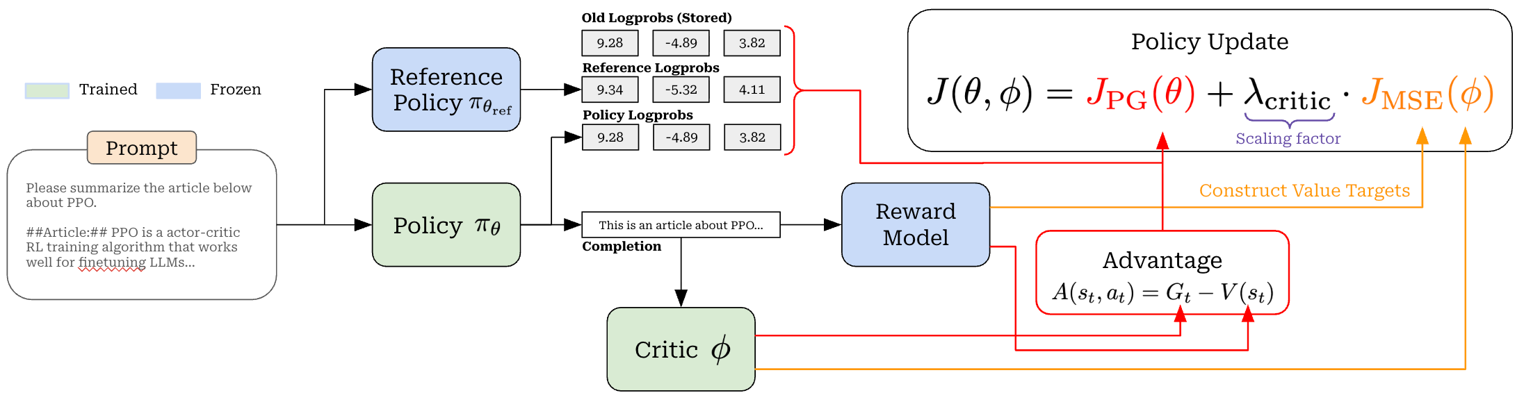
As discussed before, the critic is typically implemented using an LLM backbone with a scalar value head. This can be a separate model initialized from our policy or a value head that shares the policy’s parameters. The critic predicts expected future returns at each token position within a sequence. Whereas reward models are fixed during RL training, the value function is on-policy by definition. In other words, the value function depends upon the current parameters of our policy and, therefore, must be continually updated throughout training. The critic is usually trained with a regression loss between its predictions and observed rewards.
“TRPO uses a hard constraint rather than a penalty because it is hard to choose a single value of β that performs well across different problems—or even within a single problem, where the characteristics change over the course of learning.” - from [5]
Trust Region Policy Optimization (TRPO) [5] is an actor-critic method that is the predecessor to PPO and lays many of the foundations for how PPO works. Put simply, TRPO aims to create an algorithm that is data efficient and does not require too much hyperparameter tuning. To do this, authors in [5] propose the constrained objective below that—under certain theoretical assumptions—can be shown to monotonically improve the policy. This objective enforces a trust region on the policy update that restricts how far the new policy can move from the old policy, thus avoiding destructive policy updates that destabilize training.
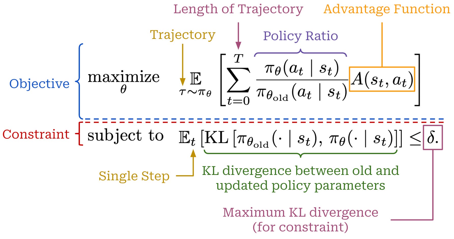
Notably, the expression above is formulated as a loss function (or objective function), rather than as a direct policy gradient expression—this is called the surrogate objective in TRPO. This naming stems from the fact that the surrogate objective is different from the standard RL training objective. In RL, we aim to maximize expected cumulative reward. However, directly maximizing the “true” objective of RL can lead to training instability. Instead, TRPO formulates the surrogate objective to maximize in place of the true objective, which improves training stability by placing a strict constraint on the size of the policy update.
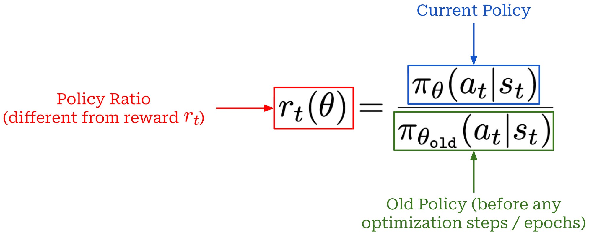
There are a few new concepts that appear with the proposal of TRPO:
The surrogate objective includes both our current policy θ and an “old” policy
θ_old. The old policy refers to the policy that was used to actually sample the rollouts, and these rollouts are then used to optimize the new candidate policyπ_θ.Action probabilities in the current policy are normalized by the probability of that action in the old policy—this forms the policy (or importance) ratio. The policy ratio, denoted as
r_t(θ), is the centerpiece of the TRPO objective.There is a constraint placed on the objective to ensure that the expected KL divergence between the new and old policies8 is less than a threshold
δ. This is a hard constraint that ensures the policy update will not be too large.
To understand the purpose of the policy ratio, we can compute the gradient of the TRPO objective; see below. A full derivation of the gradient is provided below for reference. As shown in the last step of the derivation, the TRPO policy gradient expression is composed of i) the same policy gradient structure we have seen before and ii) an importance ratio between the current and old policies.
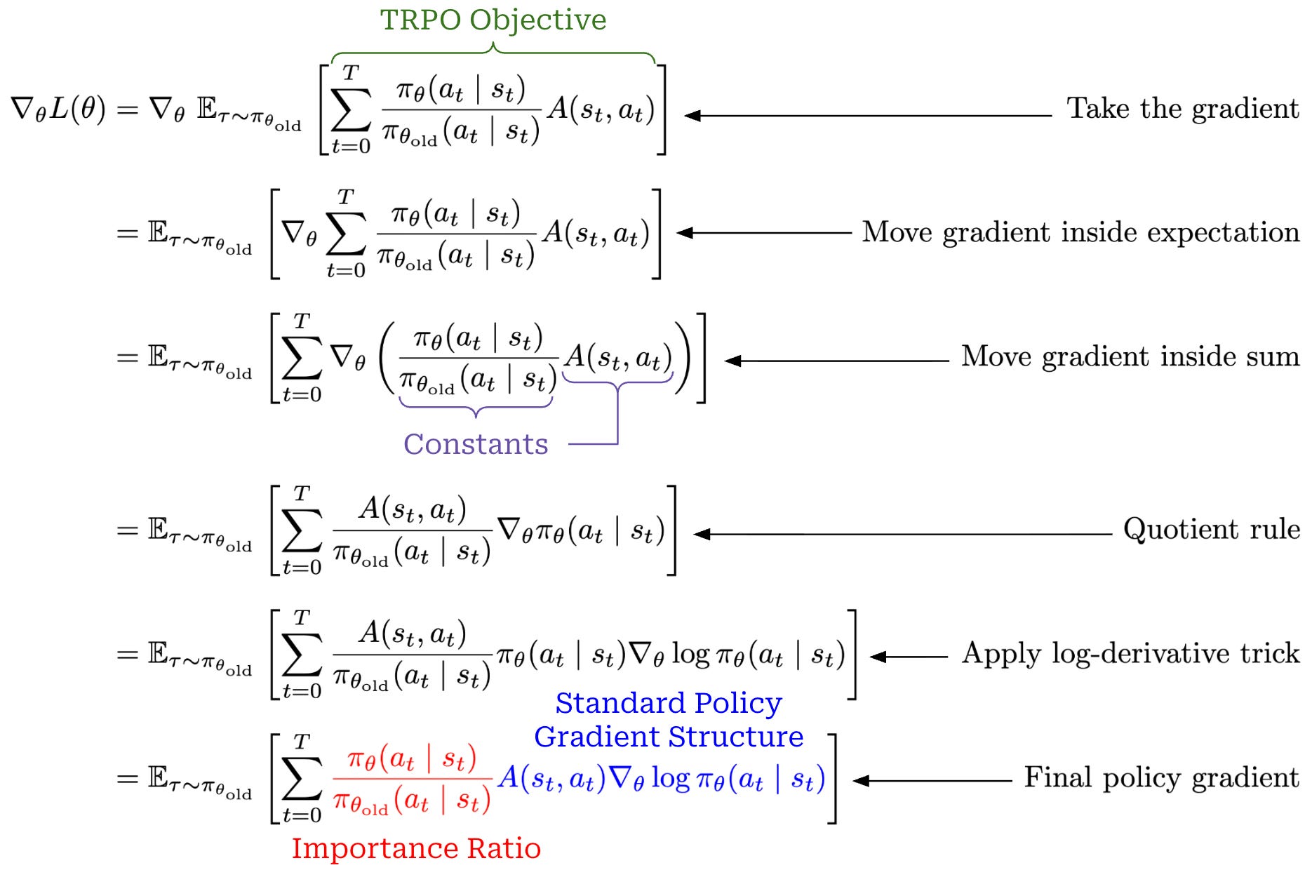
The rollouts used in the TRPO objective are sampled from the old policy π_old, and our goal is to optimize the new candidate policy π_θ. Notably, these policies may assign different probabilities to sampled actions. To account for differences in action probabilities between these policies, TRPO uses an importance ratio to reweight the sampled actions. Here, we should note that this is exactly the same importance sampling concept introduced earlier in the overview: we are evaluating the TRPO objective with π_θ using the rollouts generated by π_old.
Proximal Policy Optimization (PPO) [6]. Although TRPO produces stable policy updates, its constrained objective is hard to optimize in practice9. To solve this issue, PPO was proposed as a simpler alternative that:
Retains TRPO's goal of preventing excessively large policy updates.
Is possible to optimize with standard gradient ascent.
Similarly to TRPO, PPO focuses on optimizing a surrogate objective and can perform multiple policy updates over sampled rollouts. To obtain the objective for PPO, we take the surrogate objective being maximized by TRPO but remove the KL constraint; see below. We will refer to this as the unclipped objective.
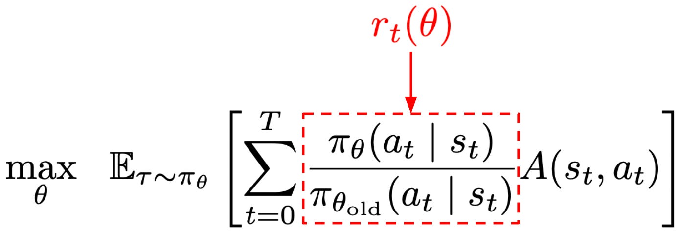
Because this objective has no hard constraint on the KL divergence, we can optimize it normally (i.e., by computing the objective above and performing gradient ascent). However, maximizing this unconstrained objective could lead to large and destructive policy updates that make the training process unstable. To solve this issue, PPO introduces a clipping mechanism into its objective that discourages large policy updates without requiring an explicit KL constraint.

The main term in the objective is unchanged, but there is an added term that clips the policy ratio to fall within the range [1 - ε, 1 + ε]. Such clipping disincentivizes the RL training process from moving the policy ratio away from a value of one, thus controlling the gap between θ and θ_old. The PPO surrogate objective takes a minimum of clipped and unclipped objectives. For this reason, the PPO objective is a pessimistic (lower) bound of the original (unclipped) objective.
More on clipping. PPO commonly performs multiple sequential policy updates using the same set of rollouts; see below. These rollouts are sampled using the old policy π_old. After the first update in this sequence, we are using data sampled from the old policy to update the parameters of our current policy θ. Therefore, the rollouts being used are slightly off-policy relative to the current policy. The importance ratio accounts for potential differences in action probabilities under these two policies. Nonetheless, PPO is still a nearly-on-policy method: rollouts are reused only a limited number of times before being refreshed.
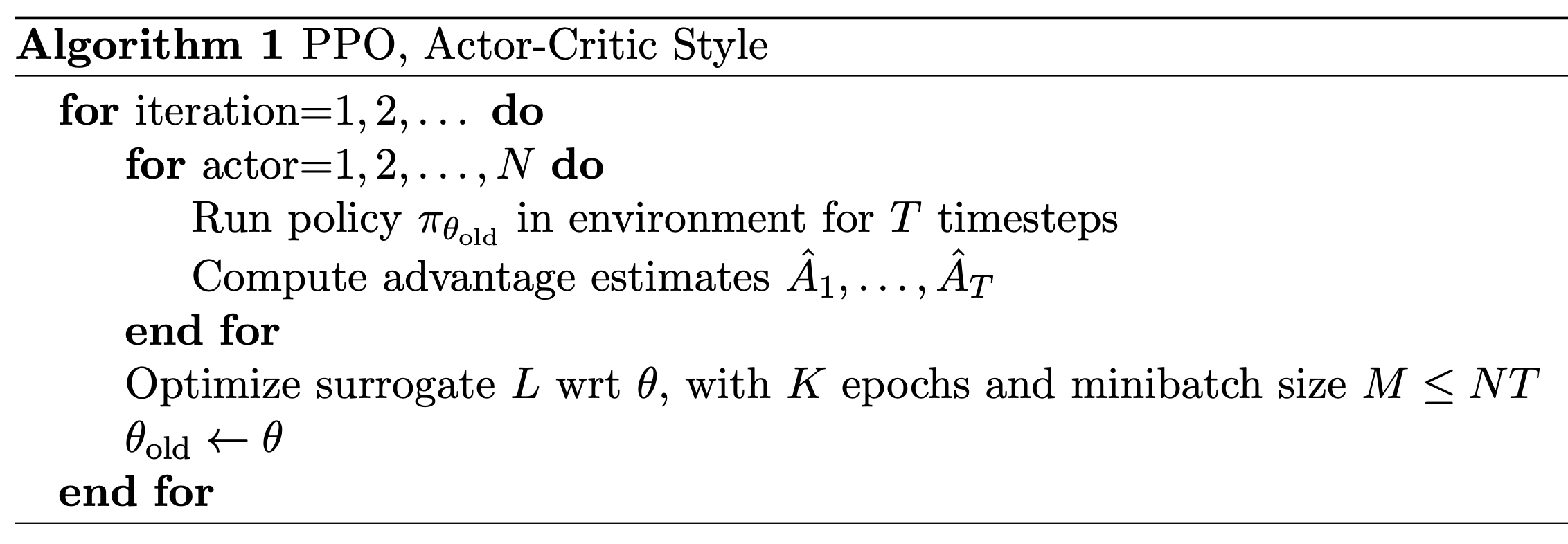
Intuitively, an importance ratio above one means that the current policy assigns greater probability to the sampled action than the old policy, while a ratio below one means that it assigns less probability. The clipping mechanism in PPO connects directly to our prior discussion of importance sampling. The unclipped policy ratio provides a standard importance-weighting correction in the surrogate objective. PPO then clips changes in the ratio only when they would improve the objective too aggressively. Such clipping introduces bias into the objective in exchange for more conservative and stable policy updates.
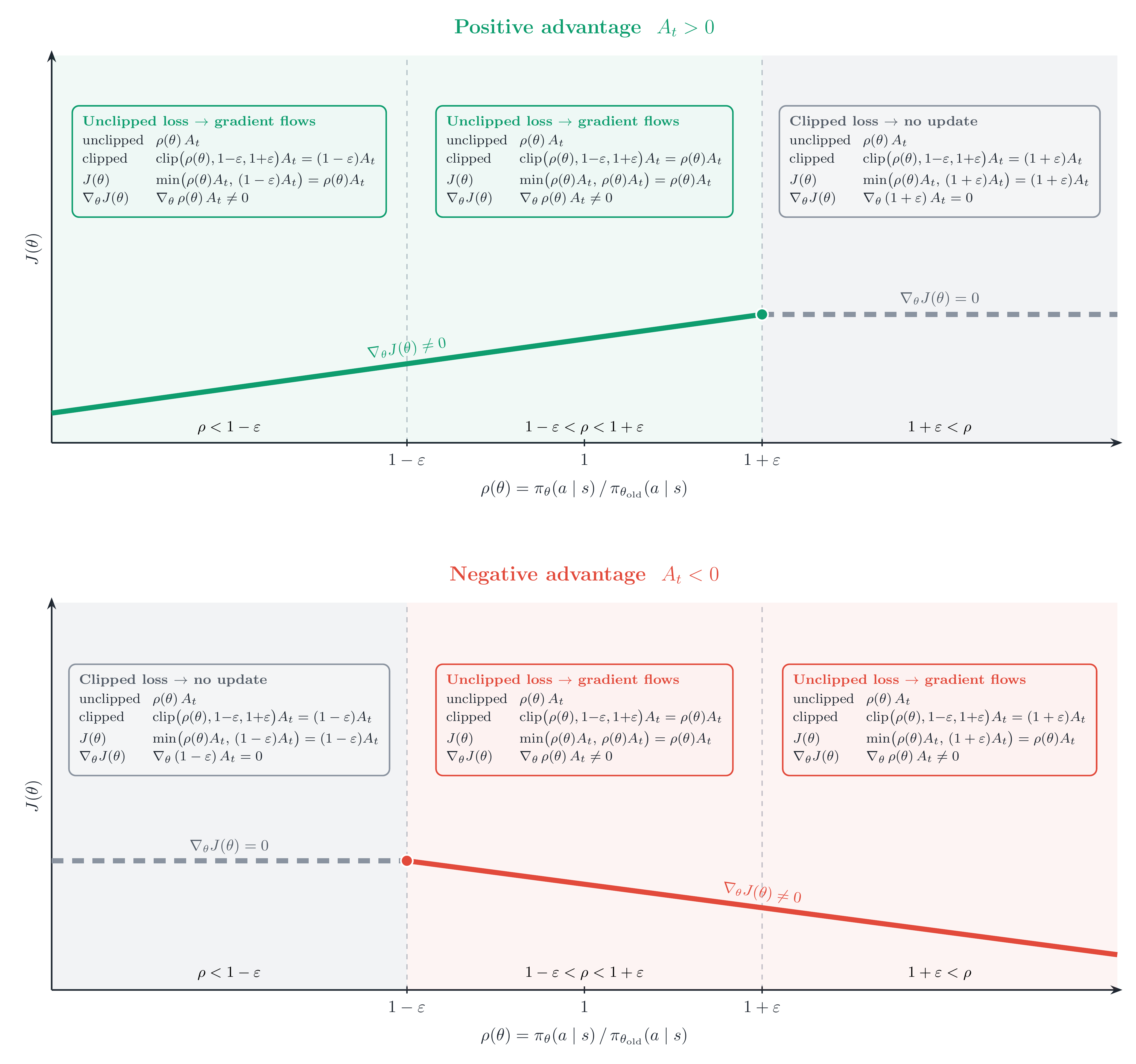
Depending upon whether the advantage is positive or negative, the behavior of clipping is slightly different; see above. The use of a minimum in the surrogate objective causes clipping to be applied in only one direction. In particular, we can arbitrarily decrease surrogate objective by moving the policy ratio far away from a value of one, but clipping prevents arbitrarily increasing the objective via the policy ratio. In this way, PPO removes the incentive for moving the policy ratio far away from a value of one when doing so would improve the objective value, thus encouraging policy updates that are more conservative.
“With this scheme, we only ignore the change in probability ratio when it would make the objective improve, and we include it when it makes the objective worse.” - from [6]
To more deeply understand the clipping logic of PPO, we can consider each of the four possible cases that can arise when optimizing the surrogate objective:
Case #1 [
A > 0,r_t(θ) ≤ 1 + ε]: advantage is positive—this is an action that we want to reinforce. Our policy ratio is below1 + ε, so we perform a normal policy gradient update to increase the probability of this action.Case #2 [
A > 0,r_t(θ) > 1 + ε]: advantage is positive again, but our policy ratio is greater than1 + ε. This means that this action is already more likely in the new policy relative to the old policy. The objective gets clipped, and the gradient with respect to further increases in the policy ratio is zero. This prevents the policy from making the action even more likely.Case #3 [
A < 0,r_t(θ) ≥ 1 - ε]: advantage is negative—this is an action we want to negatively reinforce (i.e., decrease probability). Our policy ratio is above1 - ε, so we perform a normal policy gradient update to decrease the probability of this action.Case #4 [
A < 0,r_t(θ) < 1 - ε]: advantage is negative again, but our policy ratio is less than1 - ε. This means that this action is already less likely in the new policy relative to the old policy. The objective gets clipped, and the gradient with respect to further decreases in the policy ratio is zero. This prevents the policy from making the action even less likely.
The policy ratio is computed between the current and old policies. The old policy is updated to match the current policy each time new data is sampled in PPO. In the context of LLMs, we perform 2-4 gradient updates (or sometimes more) for each batch of data, so the old model is updated frequently. The clipping operation in PPO, therefore, encourages conservative updates for a particular batch of data.
Policies in PPO. Importantly, there are multiple different policies present in the PPO objective. The old policy π_old refers to the policy used to generate the rollouts being used in the current batch, and it appears in the importance ratio for PPO. This old policy is frequently refreshed each time we sample new rollouts. In contrast, the reference policy π_ref is frozen throughout RL training and is usually equal to the policy prior to the beginning of the RL training process. The reference policy is used for KL regularization. Both old and reference policies work in tandem to control the RL optimization process:
The importance ratio
π_θ/π_oldis used to correct mismatches between old rollouts and the current policy.The KL divergence with respect to
π_refis used to discourage excessive drift away from the reference policy.
PPO implementation. To make each of these ideas more concrete, we have implemented PPO in PyTorch pseudocode below. Unlike the completion-level REINFORCE implementation shown before, this PPO implementation adopts a token-level MDP formulation—we compute a separate return and advantage for every token. This implementation also includes several other key components:
Computing a sampled KL penalty between the rollout policy and a reference model, then directly subtracting this penalty from the per-token reward. By default, most implementations of PPO incorporate the KL penalty into the reward rather than adding it into the surrogate objective. Notably, the KL-adjusted reward is computed once when the rollouts are sampled and remains fixed across the multiple policy updates performed by PPO.
Using a learned critic to compute the advantage and training this critic via an MSE loss alongside the policy itself.
Computing the policy ratio with respect to the old model and performing multiple policy updates—controlled by
num_ppo_epochs—over the same rollouts sampled from the old model before the first update.Computing the clipped PPO loss. Notably, we take the negative of this loss because PyTorch performs gradient descent (not ascent) by default.
Aggregating or averaging the token-level PPO loss across a batch of sequences. As we will see in future sections, there are many ways to aggregate the loss in a batch, and the exact approach that we use can have a non-negligible impact on model performance.
One interesting detail we see here is that—despite the PPO loss using token probabilities and not log probabilities—we choose to work with token log probabilities and exponentiate them instead of using raw probabilities when computing the policy ratio. This is a commonly-used numerical stability trick.
import torch

# B - batch size
# L - sequence length
# V - vocabulary size

# constants
kl_beta = 0.1
critic_weight = 0.5
ppo_eps = 0.2
num_ppo_epochs = 4

# sample completions from old policy
# compute (trajectory-level) rewards
with torch.no_grad():
    completions = policy.generate(prompts)
    rewards = reward_model(prompts, completions) # (B,)

# input_ids contains prompt + completion tokens
input_ids = torch.cat([prompts, completions], dim=-1)  # (B, L)

# causal shift
sampled_ids = input_ids[:, 1:]                   # (B, L-1)

# completion_mask: (B, L-1)
# masks out prompt and padding tokens

# get logprobs from old policy (policy that generated the rollout)
# these remain fixed during all PPO updates on this batch
with torch.no_grad():
    old_logits = policy(input_ids)               # (B, L, V)
    old_logits = old_logits[:, :-1, :]           # (B, L-1, V)

    old_per_token_logps = torch.log_softmax(
        old_logits, dim=-1
    )
    old_per_token_logps = old_per_token_logps.gather(
        dim=-1,
        index=sampled_ids.unsqueeze(-1)
    ).squeeze(-1)                                # (B, L-1)

# get logprobs of the same actions under reference policy
with torch.no_grad():
    reference_logits = reference_policy(input_ids)
    reference_logits = reference_logits[:, :-1, :]

    reference_per_token_logps = torch.log_softmax(
        reference_logits, dim=-1
    )
    reference_per_token_logps = reference_per_token_logps.gather(
        dim=-1,
        index=sampled_ids.unsqueeze(-1)
    ).squeeze(-1)                                # (B, L-1)

# compute critic values for the rollout
with torch.no_grad():
    old_values = critic(input_ids)[:, :-1]       # (B, L-1)

# compute per-token rewards
# per-token sampled KL penalty
per_token_kl = (
    old_per_token_logps - reference_per_token_logps
) * completion_mask

per_token_rewards = -kl_beta * per_token_kl      # (B, L-1)

# add outcome reward to final completion token
positions = torch.arange(
    completion_mask.size(1),
    device=completion_mask.device,
)
last_token_idx = (completion_mask * positions).argmax(dim=-1)

per_token_rewards[
    torch.arange(per_token_rewards.size(0)),
    last_token_idx
] += rewards

# compute reward-to-go / return for each token
returns = torch.flip(
    torch.cumsum(
        torch.flip(per_token_rewards, dims=[-1]),
        dim=-1,
    ),
    dims=[-1],
)                                                # (B, L-1)

# compute token-level advantages
advantages = returns - old_values                # (B, L-1)

# perform multiple PPO updates over same rollout data
for _ in range(num_ppo_epochs):

    # policy forward pass
    logits = policy(input_ids)                   # (B, L, V)
    logits = logits[:, :-1, :]                   # (B, L-1, V)

    # get logprobs of actions from current policy
    per_token_logps = torch.log_softmax(logits, dim=-1)
    per_token_logps = per_token_logps.gather(
        dim=-1,
        index=sampled_ids.unsqueeze(-1)
    ).squeeze(-1)                                # (B, L-1)

    # compute policy ratio
    policy_ratio = torch.exp(
        per_token_logps - old_per_token_logps
    )                                            # (B, L-1)

    # compute clipped policy ratio
    clipped_policy_ratio = torch.clamp(
        policy_ratio,
        min=1.0 - ppo_eps,
        max=1.0 + ppo_eps,
    )

    # compute PPO clipped policy loss
    policy_loss = -torch.min(
        policy_ratio * advantages,
        clipped_policy_ratio * advantages,
    )                                            # (B, L-1)

    # compute critic/value loss
    values = critic(input_ids)[:, :-1]           # (B, L-1)
    critic_loss = (values - returns) ** 2         # (B, L-1)

    # aggregate losses across completion tokens
    policy_loss = (
        (policy_loss * completion_mask).sum(dim=-1)
        / completion_mask.sum(dim=-1)
    ).mean()

    critic_loss = (
        (critic_loss * completion_mask).sum(dim=-1)
        / completion_mask.sum(dim=-1)
    ).mean()

    # combine policy + critic losses with critic weight
    loss = policy_loss + critic_weight * critic_loss

    # update policy and critic
    optimizer.zero_grad()
    loss.backward()
    optimizer.step()
Again, this implementation uses an outcome reward formulation given that this is a common setup for LLMs—every token has a KL penalty and only the final token receives an outcome reward. However, we can support process rewards by adding these rewards into the per_token_rewards at corresponding positions.
Generalized Advantage Estimation (GAE) [7]. The above PPO implementation uses a simple advantage estimation that takes the difference between the return and predicted value function. In practice, however, most PPO implementations estimate the advantage using GAE [7]. A full explanation of GAE can be found here, but we will cover the key details of the approach in this section. GAE builds upon the concept of a temporal difference (TD) residual; see below.
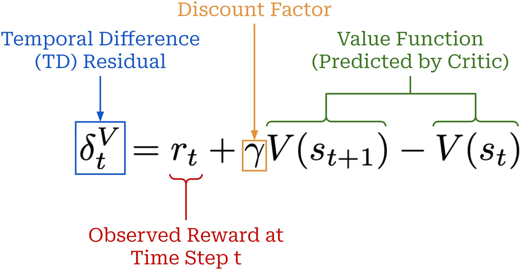
The TD residual uses per-token value predictions from the critic to form a one-step estimate of the advantage. Specifically, the TD residual compares the current value estimate V(s_t) against a one-step target made up of the true reward at this step r_t and the predicted value of the next state V(s_t+1)—this is a one-step estimate of how much better a sampled action was than expected. The TD residual only uses a small amount of actual reward information (i.e., the reward at step t) and an imperfect approximation of the value function to estimate the advantage, leading to a biased estimate. To solve this issue, we can generalize the single-step TD residual to form a series of N-step advantage estimators; see below.
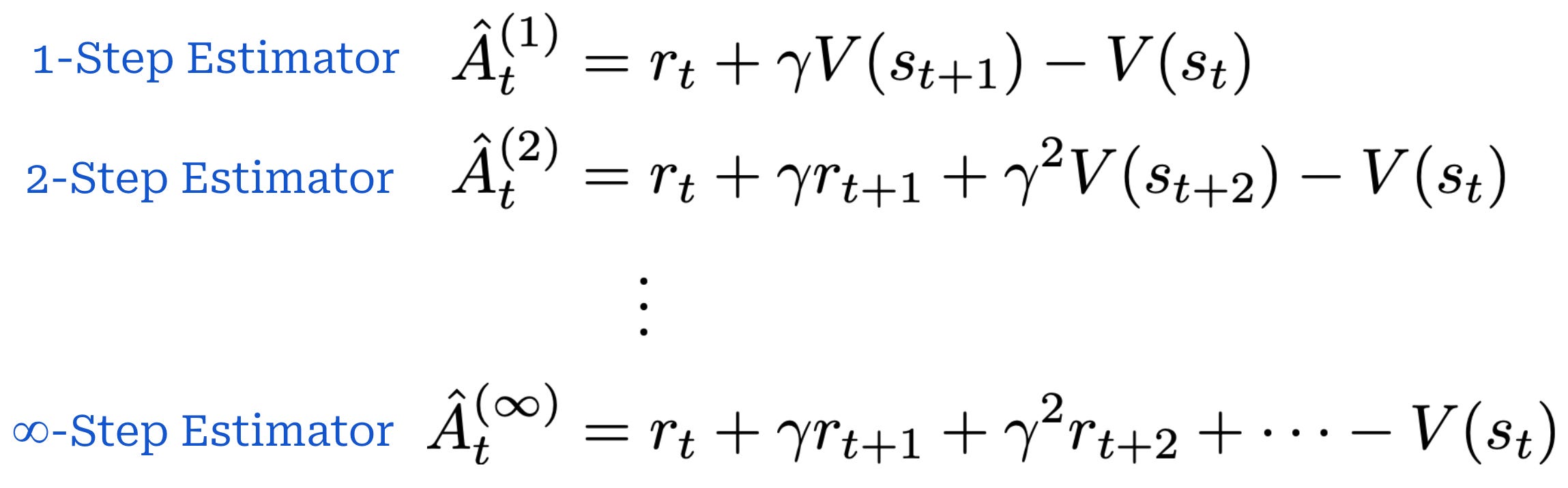
N-step advantage estimatorsSimilarly to the single-step TD residual, advantage estimators with lower values of N have low variance but high bias. As we increase the value of N, however, we are incorporating more exact reward information into the advantage estimate, thus lowering the bias (and, in turn, increasing variance). GAE tries to find a balance between these two ends of the spectrum by i) using all values of N and ii) computing an exponentially weighted combination with mixing weight λ over all of these advantage estimates; see below.
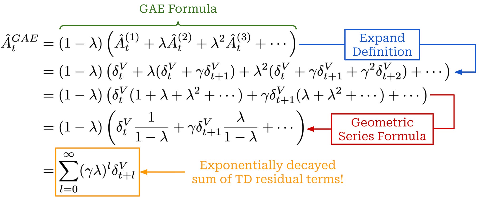
The value of λ ∈ [0, 1] controls the bias variance tradeoff. We can toggle the value of λ in GAE as needed to stabilize the training process—a common setting is λ = 0.95. For example, if training is unstable, we can decrease λ to yield lower variance policy updates. An example implementation of GAE is provided below.
import torch

# B - batch size
# L - completion length

gamma = 1.0
gae_lambda = 0.95

# per-token rewards and critic values
# per_token_rewards: (B, L)
# old_values: (B, L)

advantages = torch.zeros_like(per_token_rewards)  # (B, L)
last_gae = torch.zeros(
    per_token_rewards.size(0),
    device=per_token_rewards.device,
)                                                # (B,)

# compute GAE backwards through each completion
for t in reversed(range(per_token_rewards.size(1))):

    # terminal state has value 0
    if t == per_token_rewards.size(1) - 1:
        next_value = 0.0
    else:
        next_value = old_values[:, t + 1]         # (B,)

    # one-step TD residual
    delta = (
        per_token_rewards[:, t]
        + gamma * next_value
        - old_values[:, t]
    )                                             # (B,)

    # accumulate GAE
    last_gae = (
        delta
        + gamma * gae_lambda * last_gae
    )                                             # (B,)

    advantages[:, t] = last_gae

# targets used to train the critic
returns = advantages + old_values                 # (B, L)
Further reading. We have covered the key components of PPO in this section, but the algorithm is quite complex, and there are many details yet to be explored. For a full overview of the topic, please see the deep dive on PPO linked below.

Group Relative Policy Optimization (GRPO) [8]
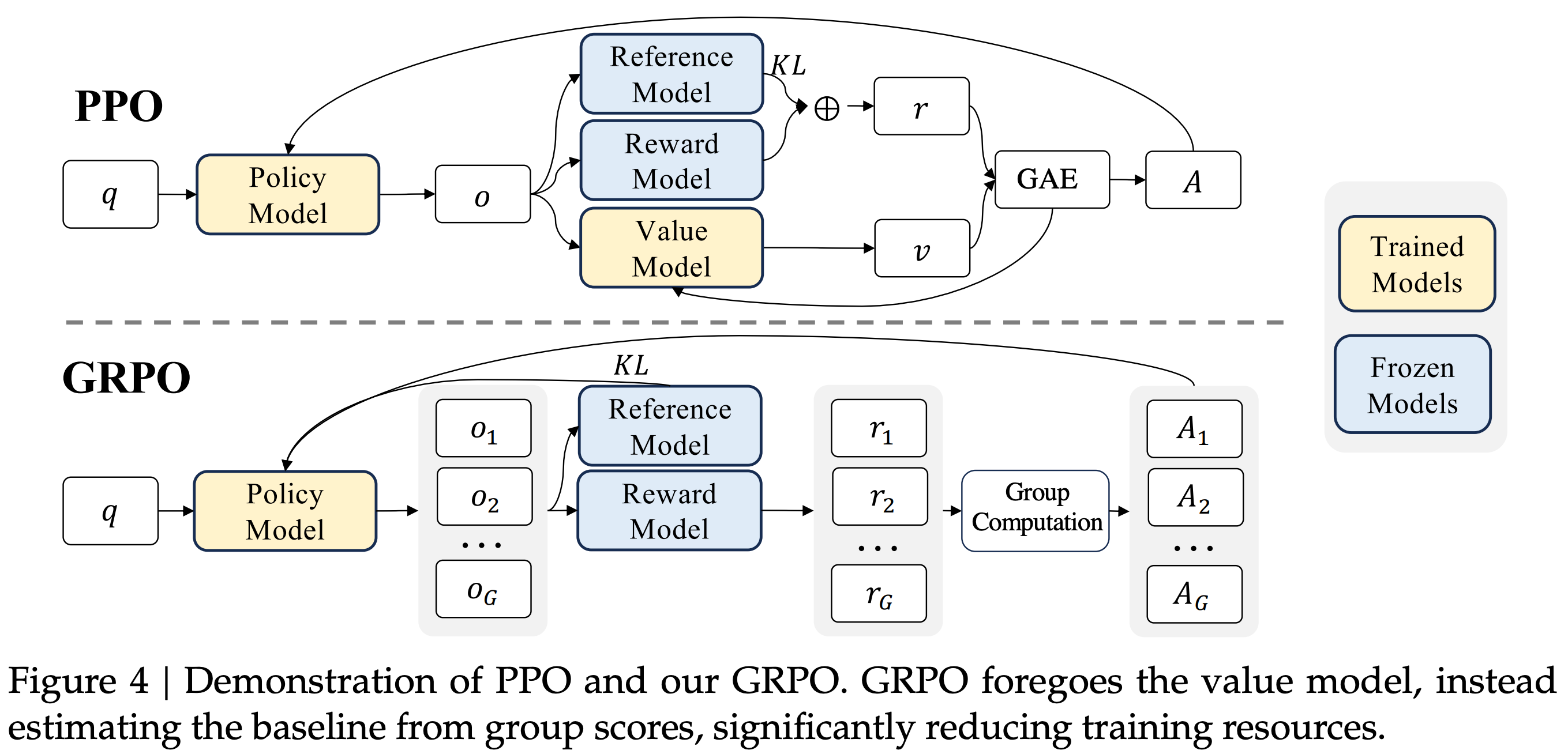
Despite its effectiveness and widespread use, PPO has practical drawbacks. Most notably, it requires training a value model—or critic—alongside the policy, which increases memory consumption, compute overhead, and training complexity. Group Relative Policy Optimization (GRPO) [8] builds on PPO by proposing a simpler technique for estimating the advantage. In particular, GRPO estimates the advantage by sampling multiple completions—or a “group” of completions—for each prompt and forming a baseline from the rewards of these completions.
“We introduce the Group Relative Policy Optimization (GRPO), a variant of Proximal Policy Optimization (PPO). GRPO foregoes the critic model, instead estimating the baseline from group scores, significantly reducing training resources.” - from [8]
This group-derived baseline replaces the role of the value function, which allows GRPO to forgo training a critic. Eliminating the critic can substantially reduce memory consumption and compute. GRPO does introduce the additional cost of sampling multiple completions per prompt, but the algorithm tends to be much simpler and lightweight relative to actor-critic methods like PPO.
Advantage estimation in GRPO. Instead of using a learned value model, GRPO estimates the advantage by sampling multiple completions for each prompt in the batch and using the formulation shown below to compute the advantage.
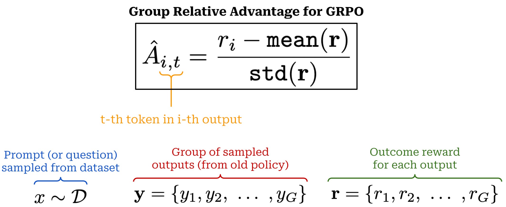
In GRPO, completions to the same prompt form a group, and we calculate the advantage relative to other rewards observed in the group—hence, the name “group relative” policy optimization! More specifically, the advantage for completion i is calculated by first subtracting the mean reward over the group from r_i, then dividing this difference by the standard deviation of rewards over the group.
Interestingly, GRPO combines aspects of the MDP and bandit formulations discussed earlier. In an outcome-reward setting, the rewards and group-relative advantages are computed at the sequence level, and every token in the completion receives the same advantage. As we will see, however, GRPO still uses a token-level objective that broadcasts this sequence-level advantage to all tokens.
“GRPO is often run with a far higher number of samples per prompt because the advantage is entirely about the relative value of a completion to its peers from that prompt.” - RLHF book
Because GRPO estimates the advantage entirely from the rewards in a group, we usually need to sample a relatively large number of completions per prompt to obtain a stable policy gradient estimate. PPO and REINFORCE can operate with only one sampled completion per prompt, but GRPO needs multiple completions to construct the group-relative baseline. Notably, this strategy is very similar to that of RLOO. Both methods avoid learning a value function and instead compare multiple completions sampled for the same prompt to compute the advantage10. In fact, we can even show that certain variants of GRPO like Dr. GRPO match the advantage estimation of RLOO up to a constant scaling factor.
Surrogate loss. Despite estimating the advantage differently, GRPO uses a surrogate loss that is nearly identical to that of PPO. Just as in PPO, π_old denotes the policy that generated the rollouts and π_θ denotes the policy being optimized. GRPO adopts the same importance ratio and applies PPO-style clipping when performing multiple updates over sampled rollouts; see below.
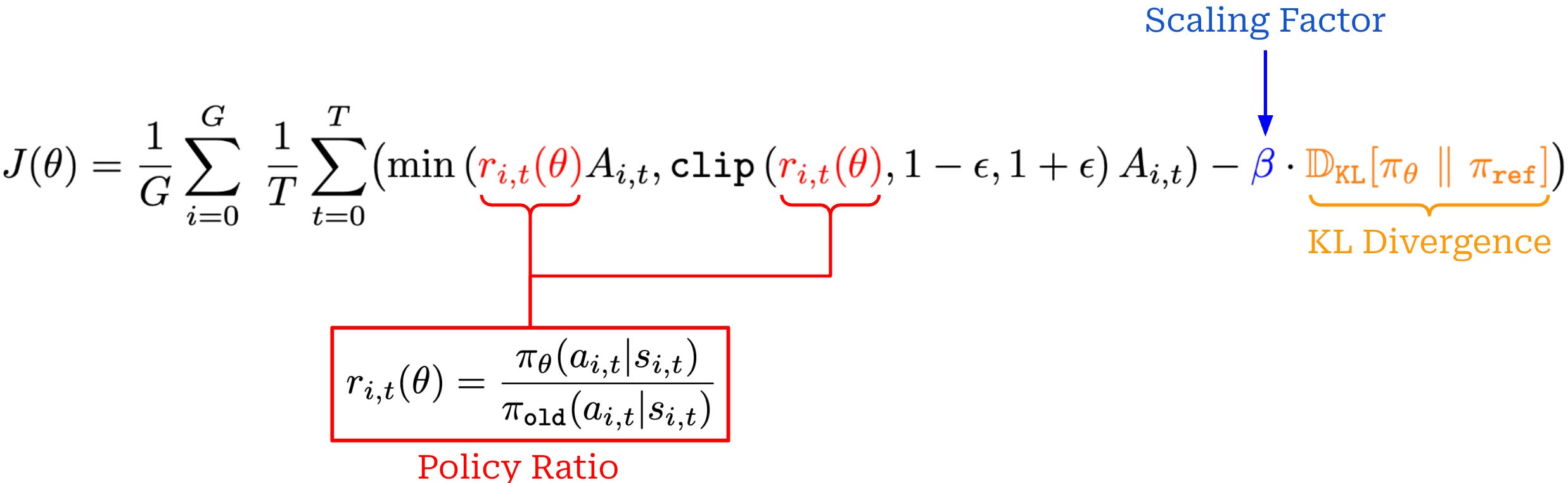
The above expression is formulated as a loss function—rather than an expectation over completions—that is averaged over tokens from multiple completions in a group. GRPO adopts a different approach for estimating the advantage but retains PPO’s methods for reusing rollouts and constraining policy updates.
We also see above that GRPO incorporates the KL penalty into the surrogate loss rather than into the reward. This choice connects to the two KL regularization strategies that were introduced earlier. In PPO, we saw that the sampled KL penalty is incorporated into the reward. We compute this KL penalty once with the old log probabilities, then detach and hold it fixed during the policy updates. In the original GRPO objective, the KL penalty is instead included directly into the (differentiable) loss function. As a result, GRPO actually recomputes the KL term during optimization, and gradients are allowed to flow through it.
Memory consumption. In PPO, we train both the policy and a learned value model or critic. Depending on the implementation, the critic can be a separate model or share a backbone with the policy. In either case, training a critic introduces additional activations, gradients, optimizer state, and compute. Additionally, we must run inference for the reference policy and (potentially) a reward model. Therefore, we are managing up to four different models in PPO—the policy, reference policy, critic, and reward model—two of which are being trained!
The need to train two models drastically increases the memory footprint of PPO. Assuming we use half precision (bf16 or fp16), we can host an LLM using ~2GB of memory for every 1B model parameters; e.g., inference with Qwen-3-32B should require ~60-70GB of memory. Notably, this calculation only accounts for loading the model’s weights into GPU memory, and memory usage can vary quite a bit depending on the maximum context length being used11.
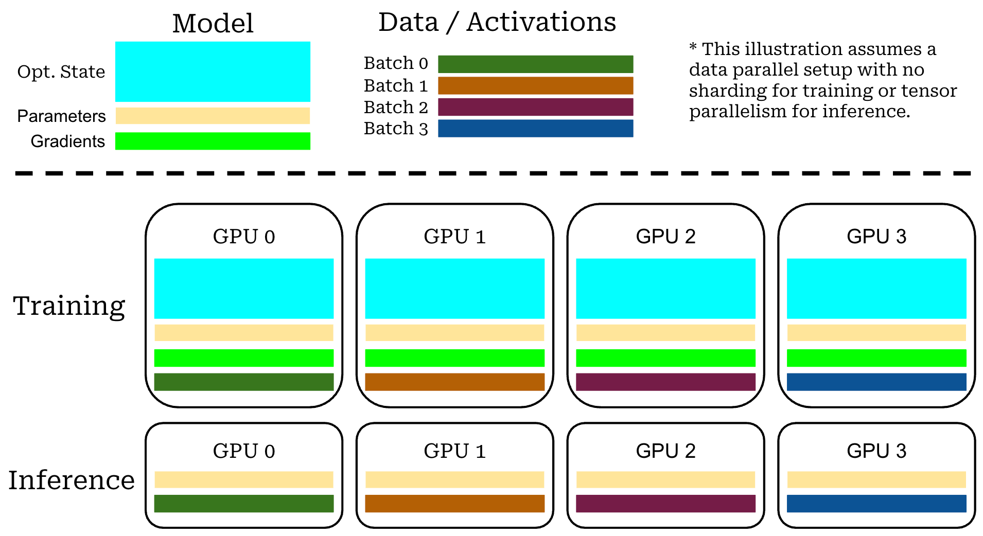
In contrast, training a model in half precision usually requires ~16GB of memory per 1B model parameters, which varies depending on the details of the training setup12. Similarly to inference, we load the model weights into GPU memory for training, but we must also store other training-related data (e.g., optimizer states and gradients). We also need enough GPU memory to store model activations during training, so memory consumption still increases with context length.
“As LMs are scaled up, computing gradients for backpropagation requires a prohibitive amount of memory—in our test, up to 12× the memory required for inference—because it needs to cache activations during the forward pass, gradients during the backward pass, and, in the case of Adam, store gradient history.” - source
With this in mind, the fact that GRPO does not use a critic not only saves on compute costs relative to PPO, but it reduces memory consumption—we are now training a single model instead of two models. Eliminating a trainable model has a much larger impact on memory consumption compared to removing a model that is only used for inference (e.g., the reward or reference models).
GRPO implementation. Finally, we will conclude our discussion of GRPO with a concrete PyTorch implementation; see below. This implementation presents two options for approximating the KL divergence. So far, the implementations we have seen use the k_1 estimator. However, authors in [8] specifically choose to adopt the k_3 estimator because it is non-negative for every sampled action and typically provides a lower-variance estimate relative to k_1 if the distributions are close. These different estimators are denoted as kl_div_k1 and kl_div_k3 in the code below, but only the k_3 estimator is used to match the setting of [8].
import torch

# B - number of prompts
# G - completions sampled per prompt
# L - sequence length
# V - vocabulary size

# constants
kl_beta = 0.1
grpo_eps = 0.2
num_grpo_epochs = 4

# sample G completions for each prompt
# compute (trajectory-level) rewards
with torch.no_grad():
    completions = policy.generate(
        prompts,
        n=G,
    )

    # repeat each prompt G times to match its completions
    repeated_prompts = prompts.repeat_interleave(G, dim=0)

    rewards = reward_model(
        repeated_prompts, completions
    )                                               # (B*G,)

# input_ids contains prompt + completion tokens
input_ids = torch.cat(
    [repeated_prompts, completions], dim=-1
)                                                   # (B*G, L)

# causal shift
sampled_ids = input_ids[:, 1:]                      # (B*G, L-1)

# completion_mask: (B*G, L-1)
# masks out prompt and padding tokens

# get log probs under policy that generated the rollout
# these remain fixed during all GRPO updates on this batch
with torch.no_grad():
    old_logits = policy(input_ids)                  # (B*G, L, V)
    old_logits = old_logits[:, :-1, :]              # (B*G, L-1, V)

    old_per_token_logps = torch.log_softmax(
        old_logits, dim=-1
    )
    old_per_token_logps = old_per_token_logps.gather(
        dim=-1,
        index=sampled_ids.unsqueeze(-1)
    ).squeeze(-1)                                   # (B*G, L-1)

# get log probs of the same actions under reference policy
with torch.no_grad():
    reference_logits = reference_policy(input_ids)
    reference_logits = reference_logits[:, :-1, :]

    reference_per_token_logps = torch.log_softmax(
        reference_logits, dim=-1
    )
    reference_per_token_logps = reference_per_token_logps.gather(
        dim=-1,
        index=sampled_ids.unsqueeze(-1)
    ).squeeze(-1)                                   # (B*G, L-1)

# compute group-relative advantages
grouped_rewards = rewards.view(B, G)                # (B, G)

reward_mean = grouped_rewards.mean(
    dim=-1, keepdim=True
)                                                   # (B, 1)

reward_std = grouped_rewards.std(
    dim=-1, keepdim=True, correction=0,
)                                                   # (B, 1)

advantages = (
    grouped_rewards - reward_mean
) / (reward_std + 1e-8)                            # (B, G)

advantages = advantages.view(B * G, 1)              # (B*G, 1)

# perform multiple GRPO updates over same rollout data
for _ in range(num_grpo_epochs):

    # policy forward pass
    logits = policy(input_ids)                      # (B*G, L, V)
    logits = logits[:, :-1, :]                      # (B*G, L-1, V)

    # get current log probs of sampled actions
    per_token_logps = torch.log_softmax(
        logits, dim=-1
    )
    per_token_logps = per_token_logps.gather(
        dim=-1,
        index=sampled_ids.unsqueeze(-1)
    ).squeeze(-1)                                   # (B*G, L-1)

    # compute policy ratio
    policy_ratio = torch.exp(
        per_token_logps - old_per_token_logps
    )                                               # (B*G, L-1)

    clipped_policy_ratio = torch.clamp(
        policy_ratio,
        min=1.0 - grpo_eps,
        max=1.0 + grpo_eps,
    )

    # compute clipped policy loss
    policy_loss = -torch.min(
        policy_ratio * advantages,
        clipped_policy_ratio * advantages,
    )                                               # (B*G, L-1)

    # compute k1 sampled KL estimate
    kl_div_k1 = (
        per_token_logps - reference_per_token_logps
    )                                                   # (B*G, L-1)

    # compute k3 KL estimate used in the original GRPO formulation
    log_ratio = (
        reference_per_token_logps - per_token_logps
    )

    kl_div_k3 = (
        torch.exp(log_ratio) - log_ratio - 1
    )                                                   # (B*G, L-1)

    # use k3 estimator in GRPO loss
    loss = policy_loss + kl_beta * kl_div_k3

    # aggregate across completion tokens
    loss = (
        (loss * completion_mask).sum(dim=-1)
        / completion_mask.sum(dim=-1)
    ).mean()

    # update policy
    optimizer.zero_grad()
    loss.backward()
    optimizer.step()
As in PPO, GRPO manages three policies with different purposes:
π_oldis used to generate rollouts and appears in the importance ratio.π_θis the current policy being optimized.π_refis the frozen reference policy used to compute the KL penalty.
Handling process rewards. Most implementations of GRPO—including our implementation presented above—use an outcome-reward setting because it is a common setting for LLMs. However, we can modify the advantage estimation in GRPO to support process rewards by:
Normalizing rewards based on the mean and standard deviation of all process rewards observed in the group.
Computing the advantage of each token as the sum of normalized rewards for following steps (i.e., the reward-to-go) in the reasoning trajectory.
When using outcome rewards, each token is assigned the same advantage by GRPO, but this approach changes when using process rewards. The advantage is estimated for each token based on rewards observed in following steps of the trajectory, which changes depending on the position of a token. Additionally, we must now consider all rewards—including multiple rewards in each trajectory—when computing the mean and standard deviation metrics for GRPO.
Further reading. For more details on GRPO, see the full writeup below, which covers the algorithm in more detail and provides a survey of related research.

GRPO++: Extensions, Improvements, and Tricks for GRPO
The GRPO algorithm exploded in popularity after the release of DeepSeek-R1 [9] as many researchers began to replicate or extend results from the paper. Despite details of the model being openly published, fully replicating the training pipeline for DeepSeek-R1 proved non-trivial, leading many subsequent works to propose tweaks to the GRPO algorithm. In this section, we will overview many of the key modifications that are now commonly adopted for better RL training.
Group Sequence Policy Optimization (GSPO) [10] modifies the GRPO objective by computing the policy ratio on a sequence level rather than at the token level. The GRPO loss introduces a misalignment between how the model is optimized and how rewards (or advantages) are assigned:
Advantage is computed at the sequence level (in an outcome reward setting).
Policy ratios—and the loss in general—are computed at the token level.
As shown in [10], per-token policy ratios tend to have high variance during RL training, which increases the variance of policy gradients and, in turn, leads to training instability. Specifically, the high variance of policy ratios can lead a single token to dominate the loss expression or even cause numerical instability during the RL training process. This problem is particularly acute when training LLMs on long sequences or using large, sparse Mixture-of-Experts models.
To protect against this variance, token-level importance ratios are clipped in the range [1 - ε, 1 + ε]. PPO-style clipping limits the contribution of token-level policy ratios that improve the surrogate objective too aggressively. When clipping becomes active for a token, the objective is constant with respect to that token’s policy ratio and, therefore, the token has zero contribution to the policy gradient. Because each token receives its own importance ratio, the variance in token-level ratios across a sequence can be high. GSPO argues that this token-level noise accumulates across long completions and can destabilize the policy gradient—we can solve this problem by using sequence-level importance ratios and clipping.
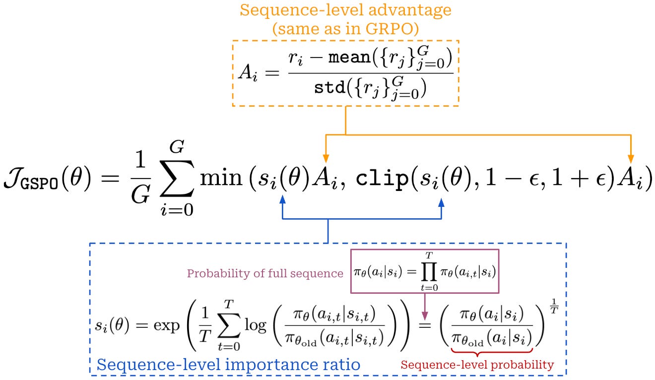
The key idea of GSPO is to compute importance ratios for the sequence rather than each token. Once we have derived the sequence-level importance ratio, the GSPO training objective is almost identical to that of GRPO; see above. We apply clipping to the sequence-level importance ratio, use the same advantage, and take a minimum of clipped and unclipped objectives at the sequence level.
The sequence-level importance ratio can be derived by factorizing the probability of a sequence into a product of individual token probabilities. However, authors in [10] choose to define the sequence-level importance ratio using the logarithmic form of a geometric mean, which is defined as shown below. This geometric mean is taken over token-level policy ratios, which normalizes the sequence-level policy ratio by the length of the sequence. By using this approach, we ensure that importance ratios for sequences of different lengths are comparable, as well as improve numerical stability—especially for long sequences—by formulating the ratio as a sum over logprobs instead of a product over raw probabilities.
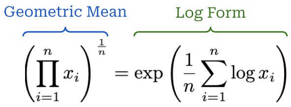
We see in [10] that GSPO improves training stability, sample efficiency, and overall performance. The stability of GSPO is found to be especially useful when training large MoE models, such as Qwen3-235B-A22B. For these reasons, GSPO was adopted in the training process for the popular Qwen 3 model series.
Decoupled Clip and Dynamic sAmpling Policy Optimization (DAPO) [11] is not a single algorithm, but rather a training recipe that is composed of several useful modifications to the vanilla GRPO optimizer. As outlined in [11], vanilla GRPO suffers from notable issues like:
Entropy collapse: the entropy of the model’s next token distribution collapses during the training process. Probability mass is primarily assigned to a single token and outputs are more deterministic.
Reward noise: the training reward is very noisy and does not steadily increase during the RL training process.
Training instability: the training process is unstable and may diverge.
To solve these issues, authors in [11] propose a suite of tricks that can be used in tandem. First, the entropy collapse problem in GRPO is shown to be caused by the fact that clipping emphasizes high probability tokens and punishes low probability (exploratory) tokens. The “clip higher” approach is proposed in [11] to solve this issue by decoupling lower and upper clipping bounds. Specifically, we clip in the range [1 - ε_low, 1 + ε_high], where ε_low = 0.2 (default setting in GRPO) and ε_high = 0.28 in [11]. Increasing ε_high prevents entropy collapse and improves overall GRPO performance; see below.
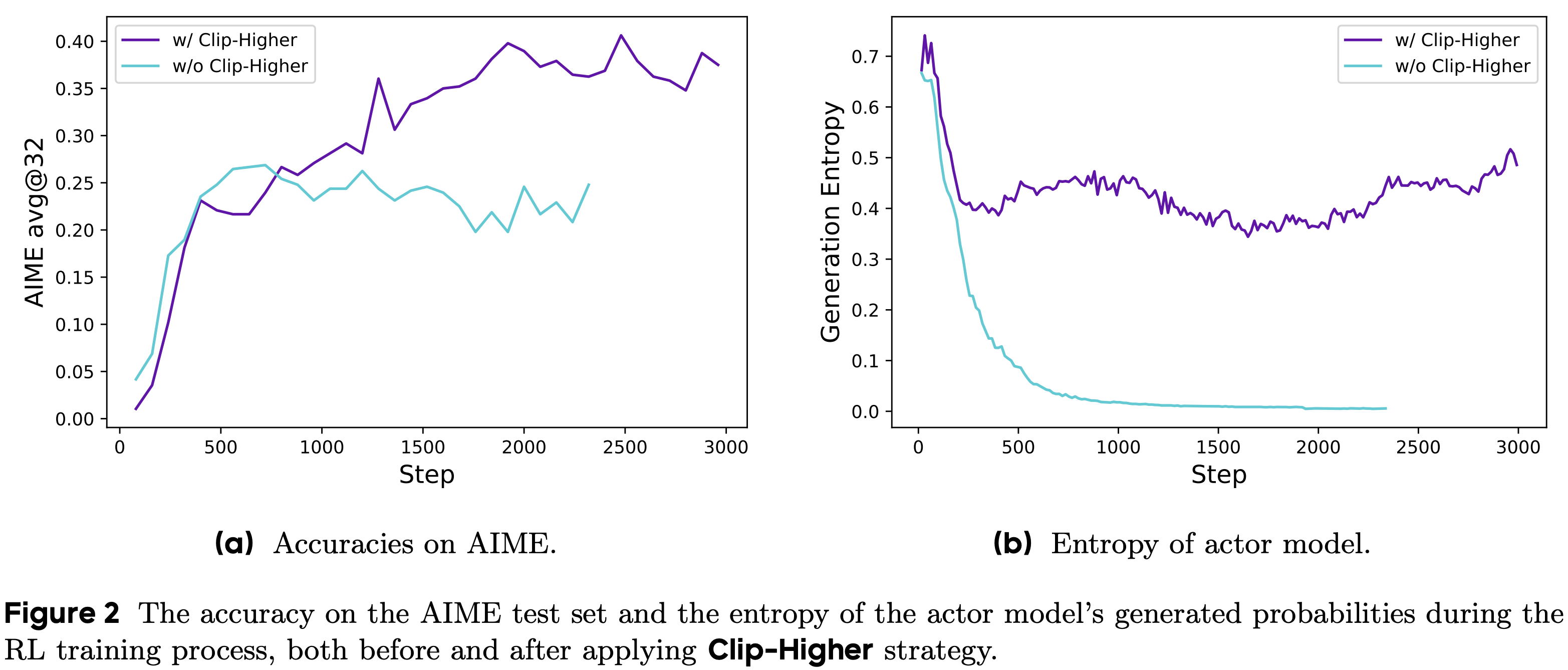
As RL training progresses, the number of samples for which all completions in a group are accurate increases. Such groups have zero advantage and, in turn, no impact on the policy gradient. As a result, these groups effectively reduce the batch size in GRPO, leading to noisier gradient estimates and degraded sample efficiency. Dynamic sampling is proposed in [11] to solve this problem by:
Filtering prompt groups where all completions receive the same reward (i.e., either perfect or zero accuracy).
Continuing to sample prompt groups until we have a full batch.
This approach can increase the cost of constructing a batch, as we dynamically continue sampling prompts until the batch is full. However, we see in [11] that this cost is offset by the improved sample efficiency of RL training; see below.
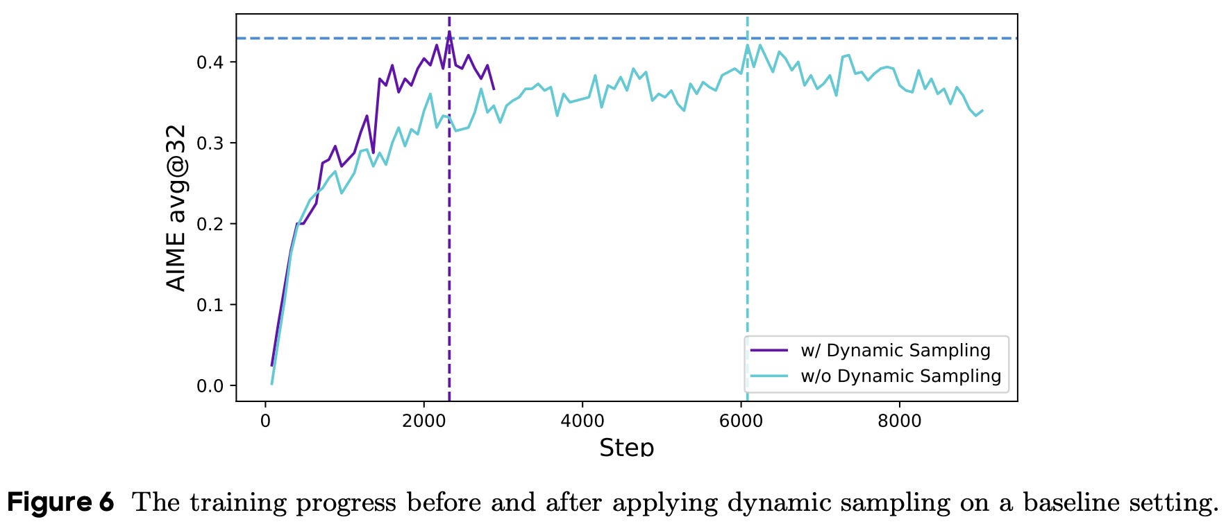
Finally, DAPO also proposes a modified loss aggregation strategy and a new approach for handling completions that exceed the maximum sequence length. Vanilla GRPO aggregates token-level losses by i) computing the average loss in each sequence and ii) averaging sequence-level losses in the batch. However, this approach introduces a subtle bias—tokens within longer sequences have relatively less contribution to the overall batch gradient. To solve this, DAPO computes a token-level loss that is simply averaged over all tokens in the batch; see below.
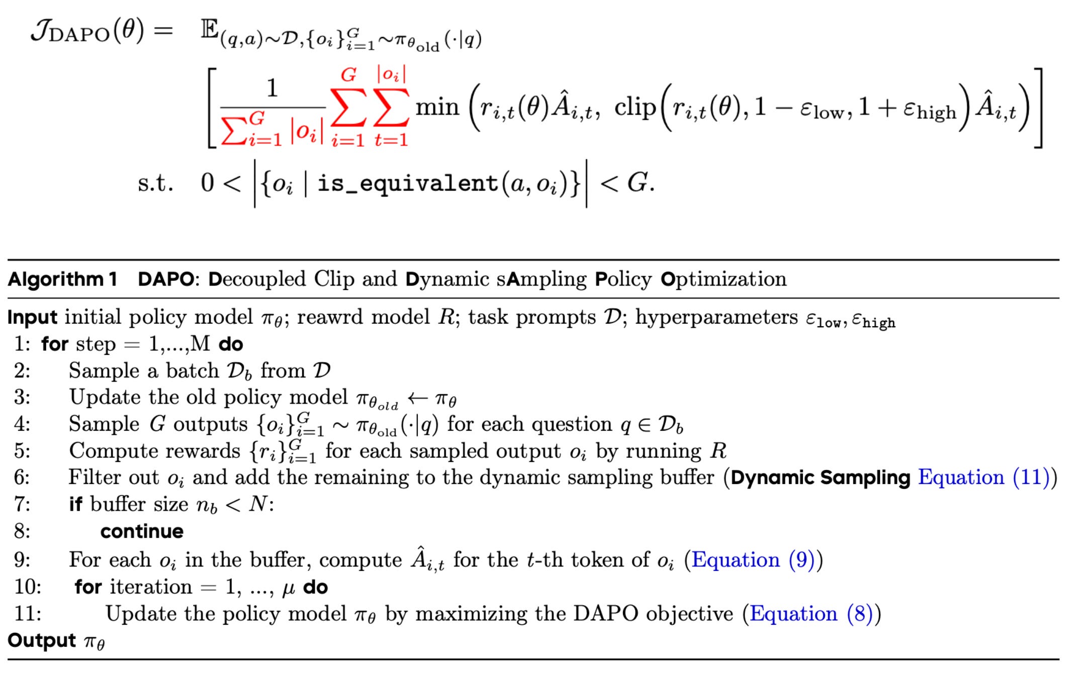
For overlong samples, DAPO uses overlong filtering, which removes truncated responses from the policy-gradient loss due to having an unreliable reward signal. Additionally, a length-based penalty term is introduced to the reward to apply a “soft” punishment to completions that are too long. Instead of assigning a hard negative reward to any completion that exceeds the maximum sequence length, authors in [11] argue that we should slowly increase the overlong penalty to its maximum value as we approach the maximum sequence length. This approach provides a smooth length penalty from which the model can effectively learn.
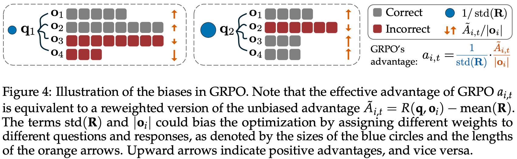
GRPO Done Right (Dr. GRPO) [12] outlined two key sources of bias that exist in the vanilla GRPO algorithm (depicted above):
Response-level length bias: GRPO normalizes the summed loss of tokens in each sequence by the total number of tokens in that sequence, leading to biased gradient updates based on the length of each response.
Question-level difficulty biases: the standard deviation term in the denominator of the advantage formulation in GRPO causes the advantage to become very large for questions that are either too easy (i.e., most responses have a reward of one) or too hard (i.e., most responses have a reward of zero).
To solve the first bias, Dr. GRPO aggregates the loss by summing token-level losses in a sequence and dividing this sum by a fixed constant MAX_TOKENS, thus removing response length from the aggregation process. The difference between this loss aggregation strategy and that of DAPO is nuanced. In DAPO, each token in the batch has an equal contribution to the gradient. As a result, DAPO still places more emphasis upon longer sequences in a batch, as these sequences have a larger ratio of total tokens (even if all tokens are weighted equally across the batch). On the other hand, replacing the sequence-level average with division by a fixed constant in Dr. GRPO effectively decouples aggregation from response lengths and, in turn, protects against length-based optimization bias.
The question-level difficulty bias is handled by removing the standard deviation term from the advantage estimator; see below. By making these two changes, Dr. GRPO improves training stability and efficiency, while making the resulting model more token efficient (i.e., responses are not artificially long).
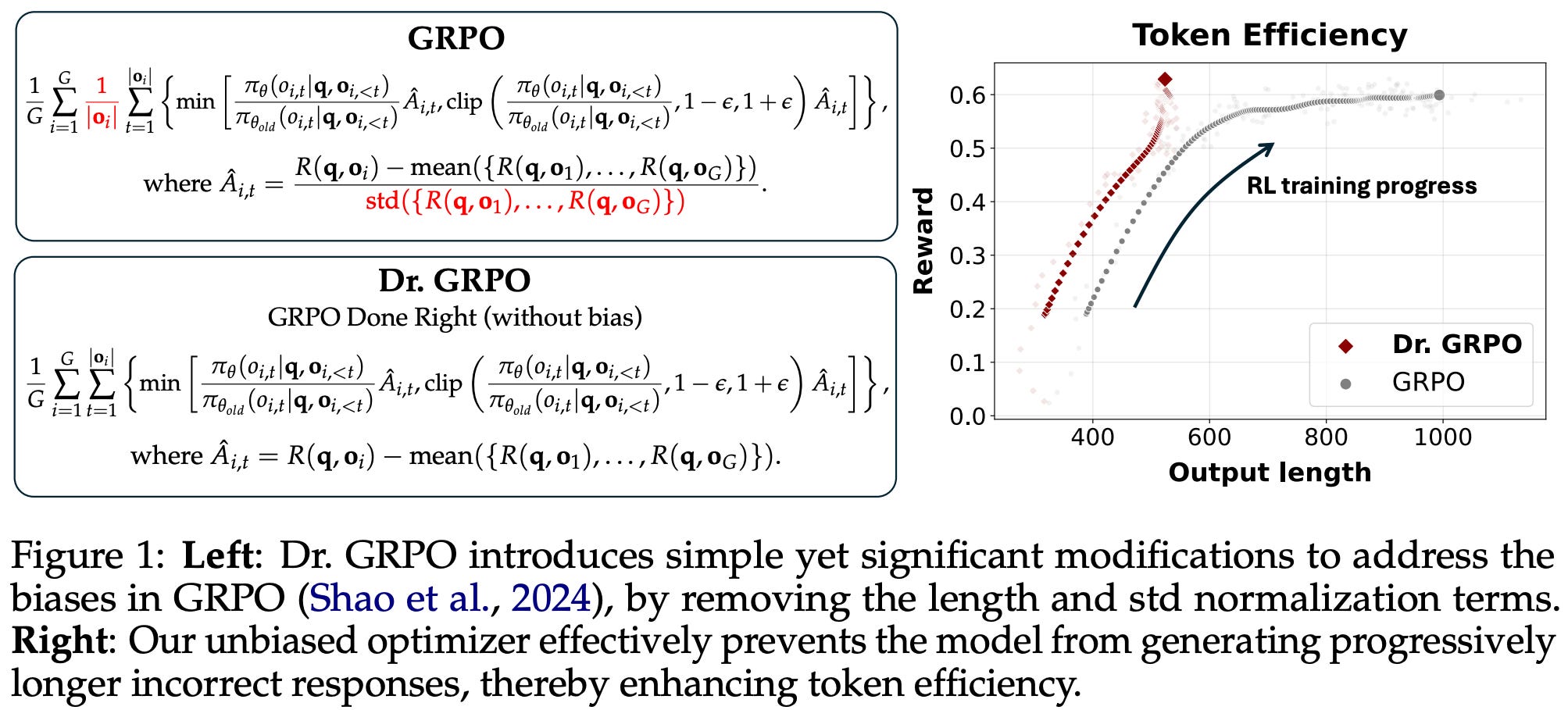
Truncated Importance Sampling (TIS) [13] attempts to address mismatches in token probabilities introduced by efficient RL training frameworks. As we know, there are two main operations that occur during RL training: i) sampling rollouts and ii) computing policy updates. In modern RL frameworks, these operations are usually handled via separate engines:
Optimized inference engines like vLLM or SGLang—often with lower precision inference (e.g.,
int8orfp8) for extra efficiency—are used to generate rollouts.Distributed training frameworks like FSDP or DeepSpeed are used to compute policy updates.
Given that generating rollouts consumes the majority of compute during RL, this approach is usually necessary—we want the inference process to be as efficient as possible. However, the use of separate engines can also introduce non-negligible differences in the token probabilities produced by each engine; see below.
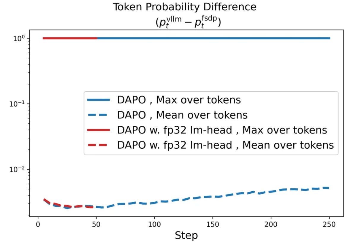
Additionally, this difference in token probabilities is not easy to fix by simply standardizing implementations across engines. Authors in [13] investigate several code interventions to decrease the gap in token probabilities with little success, and this process would have to be repeated for every combination of engines used for RL training. Instead, a more flexible approach is proposed in [13] that uses an importance sampling term to automatically correct for this engine mismatch during RL within the policy gradient expression. The exact expression is shown below and is formulated as a REINFORCE-style policy update.
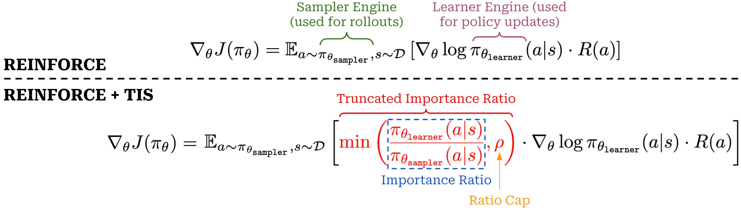
The above expression explicitly uses a different engine for sampling rollouts (sampler) and computing policy updates (learner). The importance ratio between these two engines is simply the quotient of probabilities from learner and sampler engines. Importantly, the importance ratio introduced by TIS is distinct from the PPO or GRPO policy ratio discussed before. PPO compares the current policy against the old policy and captures policy staleness introduced by optimization. Instead, TIS compares probabilities produced by learner and sampler engines in the RL infrastructure, aiming to correct system mismatches that may exist even when engines use the same model parameters.
In [13], authors truncate this importance ratio by capping it at a maximum value ρ. This differs from the clipping in PPO or GRPO in two important ways:
TIS directly truncates the importance ratio: The ratio is replaced by
min(r_t, ρ)and this truncated value is used to weight the policy-gradient term. In PPO or GRPO, by contrast, we construct both clipped and unclipped surrogate objectives and take their minimum, so a policy ratio outside the clipping interval may not be automatically clipped.TIS uses a one-sided upper bound: ratios above
ρare capped to prevent extreme up-weighting. In contrast, PPO and GRPO use a two-sided clipping interval, but the minimum in the objective makes this clipping directional—the upper bound is active for positive advantages, while the lower bound is active for negative advantages.
The practical application of TIS is quite simple—we just compute the truncated importance ratio and multiply our policy gradient expression by this ratio. As shown below, including this importance ratio in the policy gradient has a huge impact on RL training stability and model performance, leading to quick adoption of TIS in popular training frameworks (e.g., verl and OpenInstruct).
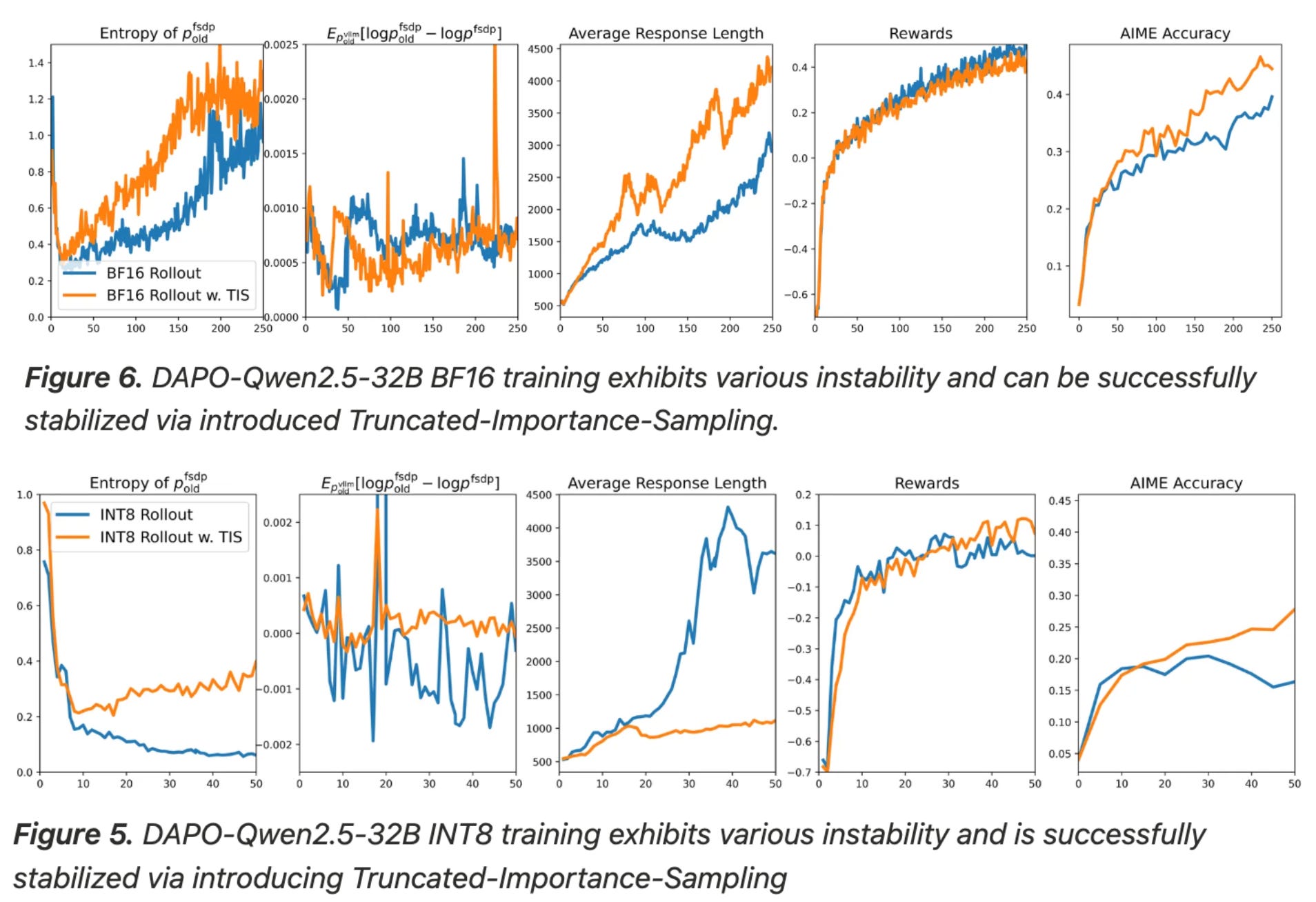
We formulated TIS above using a sequence-level importance ratio with REINFORCE. However, we can also create a token-level formulation with PPO or GRPO; see below. As we can see, the truncated importance ratio is computed in addition to the other components of the PPO-style policy gradient expression. We then multiply the existing expression by this correction term, and this can be done either at the sequence level—similarly to the gradient expression used by GSPO—or at a token level—as in the normal expression for PPO or GRPO.

Token-level TIS is commonly used in practice because it integrates nicely with PPO and GRPO objectives and is relatively simple to implement. However, recent analyses argue that:
Token-level importance ratios introduce bias relative to a sequence-level importance-sampling formulation.
Sequence-level importance ratios tend to yield higher variance.
Therefore, neither choice is clearly superior—this is a bias-variance tradeoff. The best formulation may depend on the exact training setup being used.
Clipped Importance Sampling-Weight Policy Optimization (CISPO) [14] is another recent RL variant that, similarly to TIS, builds upon a REINFORCE-style objective with an added importance ratio. When using a PPO-style clipping approach, we know any token that is clipped from the objective has no contribution to the policy gradient. In [14], authors observe empirically that the important “fork” tokens in the model’s reasoning trace (e.g., “aha” or “wait”) are rare and are initially assigned low probabilities in the base model. Due to the importance of these tokens, their probability usually increases drastically after the first policy update, leading these tokens to have a very large importance ratio—that is then clipped by the PPO objective—for subsequent policy updates.
“We found that tokens associated with reflective behaviors… were typically rare and assigned low probabilities by our base model. During policy updates, these tokens were likely to exhibit high [importance ratio] values. As a result, these tokens were clipped out after the first on-policy update, preventing them from contributing to subsequent off-policy gradient updates… These low-probability tokens are often crucial for stabilizing entropy and facilitating scalable RL.” - from [14]
As a result, important fork tokens are usually masked from the PPO-style loss after the first policy update for a batch of data. Although this masking may not always be an issue (i.e., most standard RL setups perform only ~2-4 updates on each batch of sampled data), MiniMax-M1 performs 16 policy updates for each batch of data. Therefore, important tokens being masked out of the loss after only one or a few updates can significantly damage training efficiency. To solve this issue, authors adopt the modified REINFORCE-style loss shown below. As we can see, CISPO adopts some of the recommendations proposed by DAPO [11] as well, including the token-level loss formulation to correct for length biases.
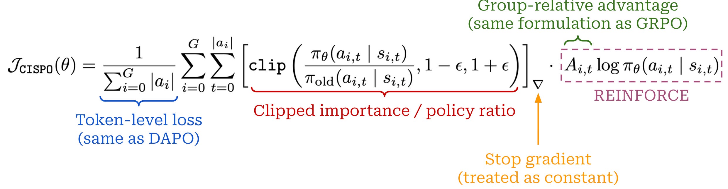
This loss formulation applies a stop gradient to the clipped importance ratio, ensuring that each token contributes to the loss even when it is clipped. Put differently, the importance ratio is used as a weight that controls the contribution of a token to the policy gradient. Clipping in CISPO puts a cap on this weight, ensuring no single token is over-amplified due to a large importance ratio.

When we look at the GRPO objective, the clipping mechanics are quite different; see above. In particular, token probabilities are only present in the importance ratio, and the gradient flows through the token probability terms inside the importance ratio. When the importance ratio is clipped, the gradient for that token is zero and there is no contribution to the policy gradient. The modified clipping approach used by CISPO ensures that all tokens contribute to the policy gradient, improving the stability and efficiency of RL; see below.
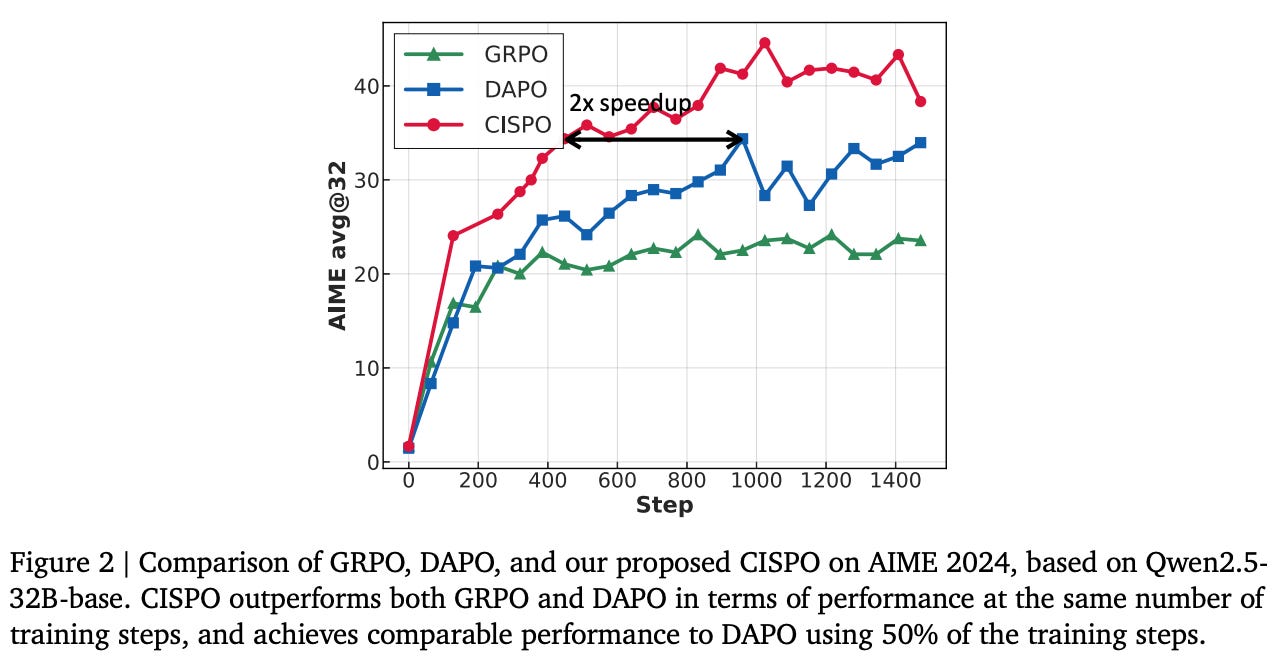
The loss formulation of CISPO and TIS look quite similar, but these algorithms—despite both using an importance ratio—aim to solve different issues. CISPO uses the same importance ratio found in PPO and GRPO. Rather than using clipping to suppress the policy gradient once a token's ratio moves outside the preferred range, however, CISPO clips the ratio and uses it as a stop-gradient importance weight. The clipped ratio controls the magnitude of a token’s contribution to the policy gradient, rather than eliminating this contribution. In contrast, TIS uses an importance ratio between training and inference engines to correct for a system-induced mismatch. Therefore, CISPO and TIS both use importance-weighted policy-gradient objectives but address different forms of mismatch.
Further reading. Although we have covered the most prominent variants and tricks for GRPO in this section, a wide variety of research has been published on this topic. Please see the link below for a full deep dive on GRPO modifications.

Advanced Research Topics in RL
We now have a deep understanding of RL fundamentals for LLMs, as well as the many RL optimizers that are used within this space. To further build upon this understanding, we will now look at more advanced topics in RL research. In this section, a variety of recent research topics will be presented, each paired with a brief explanation of the space and a link to a full overview on the topic. In prior sections of this overview, we focused on fundamental concepts and established knowledge in RL research. Now, we will deepen our understanding of RL by exploring the open questions that are shaping recent trends in AI research.
Online versus Offline RL for LLMs
One of the most important design choices in RL is the frequency with which we sample fresh data for training. Online RL algorithms—such as PPO, GRPO, and other algorithms we have seen in this overview—continually generate on-policy completions during training, while offline algorithms like DPO train on a fixed dataset. Online RL is more difficult to orchestrate relative to offline methods, but studies consistently show that training with on-policy data has a positive impact on model performance. On-policy samples are especially important when working in difficult settings where responses that receive high rewards are not likely in the initial policy. To perform well in this case, the model must be able to actively explore new behavior, which is difficult when the training dataset is fixed.

Interestingly, the choice between online and offline training is not completely binary. Studies show that much of the benefit of online RL can be recovered with semi-online approaches that periodically refresh training data with on-policy samples. Additionally, recent work in asynchronous RL training infrastructure must handle cases where rollouts used in training are partially off-policy. More specifically, several policy updates could be performed before a long-running rollout finishes, leading to the incorporation of stale data into training that must be handled properly. Across this work, the key takeaway is that fresh, on-policy data is an important ingredient for achieving good results with RL training.
Continual Learning with RL for LLMs
Continual learning refers to the ability of a model to learn new tasks over time without degrading its performance on previously-learned tasks. Historically, continual learning has been difficult for neural networks due to catastrophic forgetting—the tendency to completely forget old data when training on new data. However, recent studies in the LLM domain show that on-policy RL is naturally robust to catastrophic forgetting, especially relative to supervised training.
For example, when sequentially training models on new tasks, RL nearly reaches the performance of multi-task training and largely maintains the general capabilities of the LLM, even without using specialized techniques (e.g., replay buffers or regularization). In contrast, SFT tends to learn new tasks well but progressively forgets old tasks throughout the training process. Such a finding suggests that we can incorporate new skills into an LLM through sequential phases of RL while largely preserving general capabilities and prior task performance; e.g., Nemotron-Cascade uses such a sequential RL pipeline.

When we dig deeper into the ability of RL to avoid forgetting, we learn that on-policy data plays a key role. In online RL, we train the model using on-policy completions, which means that the data used for training is sampled from the model itself. As a result, policy updates remain close to behaviors that are already plausible under the current model. Empirically, models trained with online RL undergo relatively little distribution shift—measured using KL divergence—from the initial model, which is strongly correlated with reduced forgetting. In contrast, supervised training on offline data forces the model to imitate fixed completions, inducing larger changes in behavior and (potentially) forgetting.
Rubric-based Rewards for RL
A large fraction of recent RL research for LLMs focuses on verifiable domains like math and code, where rewards can be computed with deterministic verifiers (e.g., exact answer matching, symbolic verification, or unit tests). Verifiable settings are attractive domains for RL because the reward can be computed efficiently and is less prone to reward hacking compared to learned reward models, thus enabling larger-scale RL training. However, many important tasks that LLMs are expected to solve—such as creative writing or scientific research—are open-ended and non-verifiable in nature. Therefore, we need some way to derive a reliable reward signal for RL training in these important domains.

Rubric-based rewards provide a promising way to generalize the benefits of RL beyond verifiable domains. To compute the reward, we first derive a rubric—or a checklist of prompt-specific quality criteria—that describes the characteristics of a good completion. We then use an LLM judge to separately evaluate each criterion and aggregate the results into a final reward. Recent work shows that this structured approach provides informative and controllable reward signals for open-ended tasks while reducing the risk of reward hacking. In particular, strong results are obtained when rubrics are prompt-specific, comprehensive, and grounded in expert guidance or high-quality reference answers.
RL Scaling Laws for LLMs
Scaling laws have traditionally been studied in the context of pretraining, where we observe smooth and predictable relationships between model performance, compute, data volume, and model size. As RL becomes an increasingly large component of the LLM training process—especially for reasoning models—a natural question is whether similar scaling trends exist for RL. Recent work shows that RL performance does scale predictably with compute. However, the scaling laws observed for RL are much messier relative to those used for pretraining.
When performing scaling analysis for RL, we usually measure performance using downstream reward or accuracy. Such metrics are variable, application-specific, and often highly dependent upon evaluation settings. In contrast, most scaling analyses for pretraining measure performance using cross-entropy loss on held-out validation data13, which provides a much smoother and more continuous metric. Similarly, consistently measuring the amount of compute used during RL training is non-trivial compared to pretraining—RL compute is split between generating rollouts and performing policy updates. For these reasons, RL scaling laws tend to be highly dependent upon the exact model, data, and training recipe being used, rather than providing a general scaling trend as in pretraining.

Despite the lack of standardization, useful findings have emerged from research on RL scaling. First, the early phase of RL training can often be extrapolated to predict performance at larger compute scales, allowing us to test training recipes efficiently and identify those that are scalable. Additionally, there are multiple ways to scale RL beyond simply increasing the number of training steps. For example, larger batch sizes, data reuse, and allocating more compute to rollouts (i.e., sampling more completions per prompt) can all improve performance. RL scaling laws provide a framework for predicting how RL training will behave at scale and deciding how to allocate a fixed compute budget in a training run.
Agentic RL
In this overview, we have mostly considered relatively simple, single-turn tasks, where the LLM receives a prompt and generates a response. However, LLM systems are becoming increasingly agentic—they reason over long time horizons, call tools, and interact with external environments. Training agentic systems with RL is fundamentally more complicated. Compared to a single completion, agentic rollouts contain multiple rounds of generation and environment interaction, including tool calls, observations, rewards, changes in state, and more. As a result, agentic RL naturally requires more sophisticated training infrastructure.

Although agentic RL is complex, there are several common design patterns and considerations that emerge from work in this space:
Designing modular tool and environment interfaces that allow arbitrary domains to be more easily incorporated into the training infrastructure.
Masking the RL objective such that only agent-generated tokens—and not environment-generated tokens (e.g., tool outputs or observations)—are included in the policy update.
Supporting intermediate process rewards to enable better credit assignment in long trajectories.
Exploring different advantage normalization techniques that are aware of the different environments included in a training batch.
Adopting asynchronous infrastructure that can handle rollouts that vary dramatically in wall-clock completion time while managing stale data and avoiding negative impacts of off-policy learning.
Scaling environment orchestration to support thousands of concurrently-running environments without centralized bottlenecks.
Agentic RL is an emerging—and quickly evolving—space. The research in this area is particularly interesting due to its multi-faceted nature. Recent work on agentic RL involves algorithms, data curation, infrastructure, and software engineering (e.g., designing the correct environment interface or trajectory schema). As one example of the broader domain, the overview below explores how world modeling can be incorporated into agentic RL training to improve an agent’s capabilities.

From Policy Gradients to Frontier RL
In this overview, we have covered the core concepts needed to understand recent RL research in the LLM domain. Starting with basic mathematical formulations, we outlined key building blocks and concepts for understanding RL, such as value and advantage functions, objectives, policy gradients, KL regularization, importance sampling, and more. We then built upon these foundations by walking through the evolution of policy gradient algorithms from the vanilla policy gradient to recently proposed variants of GRPO. To conclude, we will now provide a summary of this progression of RL algorithms, focusing on the key changes introduced by each of the approaches that we have covered.
Policy gradients. We began our discussion with the VPG, which provides the core idea behind nearly every algorithm in this overview. Put simply, the VPG aims to increase the probability of actions that lead to good outcomes and decrease the probability of actions that lead to bad outcomes. Mathematically, this takes the form of a log-probability gradient multiplied by a learning signal such as a return or advantage. Although modern RL algorithms tend to be more complicated than the VPG, this same basic structure underlies them all.
REINFORCE concretely instantiates the VPG. The VPG is expressed as an expectation over trajectories. In practice, we can take a Monte Carlo estimate of this expectation by sampling rollouts and averaging our policy gradient expression over these rollouts—this is exactly the idea behind REINFORCE. A Monte Carlo estimate of the policy gradient tends to have high variance, but we can reduce this variance by using an action-independent baseline. Additionally, we can use a REINFORCE variant like RLOO, which constructs a prompt-specific baseline by comparing multiple completions to the same prompt.
PPO = powerful advantage estimation + conservative updates. To reduce the variance of our policy-gradient estimate, we can use an actor-critic framework that uses a learned value model—or critic—to estimate the value function and construct an advantage estimate. One canonical example of an actor-critic algorithm is PPO. Beyond using a critic to estimate the advantage, PPO uses importance ratios and clipping to allow multiple policy updates to be performed over sampled rollouts while still protecting against large or destructive policy updates. In PPO, many concepts we learned in this overview—value functions, importance sampling, advantage estimation, and KL divergence—come together.
GRPO simplifies PPO by removing the critic. PPO is effective and widely used in LLM research, both in early work on RLHF and recent work on large-scale RL training. However, actor-critic frameworks are complex and expensive because they require training a critic alongside the policy. To solve this issue, GRPO avoids learning a value model by sampling multiple completions for each prompt and estimating the advantage by comparing each completion’s reward to others in the group. Such an approach connects directly to the group-based baselines used in RLOO but retains PPO-style importance ratios and clipping. The result is a simpler RL optimizer that trades additional compute spent on sampling rollouts for a simpler and more lightweight optimization process—a property that made GRPO very popular in large-scale RL training for reasoning models.
Beyond vanilla GRPO. Methods like DAPO, Dr. GRPO, GSPO, TIS, and CISPO do not completely reinvent the policy gradient. Instead, they refine seemingly small details of existing policy gradient algorithms that are important at scale. Specific modifications that are targeted include:
How the loss is aggregated over the batch.
How rewards are normalized to obtain the advantage estimate.
Which samples are included in a batch.
How clipping is applied to the importance ratio.
Whether importance ratios are computed per-token or per-sequence.
How mismatches between inference and training engines are handled.
These ideas emerged from an effort by the AI research community to make GRPO—and large-scale RL training more generally—more stable, efficient, and effective.
Looking forward. After tracing the evolution of policy gradient algorithms, we concluded this overview by exploring a broad set of advanced research topics in RL. Despite the enormous progress made in recent years, RL remains full of open questions around data, rewards, scaling, continual learning, long-horizon reasoning, agents, and much more. Together, these topics form one of the key frontiers within LLM research. In this overview, we have developed the conceptual foundation needed to meaningfully contribute to this frontier. My sincere hope is that, by reading this overview, readers will be enabled to ask their own questions, test new ideas, and—eventually—push the boundaries of RL.
New to the newsletter?
Hi! I’m Cameron R. Wolfe, Deep Learning Ph.D. and Staff Research Scientist at Netflix. This is the Deep (Learning) Focus newsletter, where I help readers better understand important topics in AI research. If you like the newsletter, subscribe, consider a paid subscription, share it, or follow me on X, Medium, and LinkedIn!
Bibliography
[1] Guo, Daya, et al. “Deepseek-r1: Incentivizing reasoning capability in llms via reinforcement learning.” arXiv preprint arXiv:2501.12948 (2025).
[2] Schulman, John, et al. “High-dimensional continuous control using generalized advantage estimation.” arXiv preprint arXiv:1506.02438 (2015).
[3] Williams, Ronald J. “Simple statistical gradient-following algorithms for connectionist reinforcement learning.” Machine learning 8.3 (1992): 229-256.
[4] Schulman, John. “Approximating KL Divergence.” Online (2020). http://joschu.net/blog/kl-approx.html.
[5] Schulman, John, et al. “Trust region policy optimization.” International conference on machine learning. Pmlr, 2015.
[6] Schulman, John, et al. “Proximal policy optimization algorithms.” arXiv preprint arXiv:1707.06347 (2017).
[7] Schulman, John, et al. “High-dimensional continuous control using generalized advantage estimation.” arXiv preprint arXiv:1506.02438 (2015).
[8] Shao, Zhihong, et al. “Deepseekmath: Pushing the limits of mathematical reasoning in open language models.” arXiv preprint arXiv:2402.03300 (2024).
[9] Guo, Daya, et al. “Deepseek-r1: Incentivizing reasoning capability in llms via reinforcement learning.” arXiv preprint arXiv:2501.12948 (2025).
[10] Zheng, Chujie, et al. “Group sequence policy optimization.” arXiv preprint arXiv:2507.18071 (2025).
[11] Yu, Qiying, et al. “Dapo: An open-source llm reinforcement learning system at scale, 2025.” URL https://arxiv. org/abs/2503.14476 1 (2025): 2.
[12] Liu, Zichen, et al. “Understanding r1-zero-like training: A critical perspective.” arXiv preprint arXiv:2503.20783 (2025).
[13] F. Yao, L. Liu, D. Zhang, C. Dong, J. Shang, and J. Gao. Your efficient rl framework secretly brings you off-policy rl training, Aug. 2025. URL https://fengyao.notion.site/off-policy-rl.
[14] Chen, Aili, et al. “MiniMax-M1: Scaling Test-Time Compute Efficiently with Lightning Attention.” arXiv preprint arXiv:2506.13585 (2025).
[15] Ahmadian, Arash, et al. “Back to basics: Revisiting reinforce style optimization for learning from human feedback in llms.” arXiv preprint arXiv:2402.14740 (2024).
Notably, this notation is used in the RLHF book, as well as other popular writeups on policy gradient algorithms. However, the R(τ) is also commonly used; e.g., in OpenAI’s spinning up in deep RL series.
Put simply, Monte Carlo estimate is just a fancy way to say that we take random samples and average over them to approximate a target value (e.g., an expectation).
Note that some of these rewards being assigned could be zero. Therefore, we can still formulate an outcome reward setting as a reward of zero being assigned at each step, followed by the outcome reward in the last step.
However, recent work on RL training for reasoning models utilizes KL penalties less frequently than prior RL training recipes for LLMs. In such large-scale RL training runs, anchoring the current policy to the reference policy may be too restrictive—we may want the policy to undergo significant change during RL training.
Adding baselines to the policy gradient does not bias our gradient estimate. This fact can be proven by using the EGLP lemma, which mandates that the baseline cannot depend on the action a_t. A state-dependent baseline does not change the expectation for the policy gradient because E[b(s_t)·∇_θ log π_θ(a_t∣s_t)] = 0.
Technically, the baseline would be the average of returns. However, we adopt the average of rewards here because we are assuming a the outcome-reward setting that is commonly used for LLMs. Additionally, a batch mean that includes the current completion—which is used in implementation of REINFORCE we show here—is not action-independent because each sample contributes to its own baseline. Therefore, this particular approach introduces bias into the policy gradient expression. As we will see, RLOO aims to fix exactly this issue by excluding the current sample from the baseline.
Note here that the KL divergence is computed with respect to the old policy—the policy used to sample data during RL—rather than the reference policy—the model from the beginning of RL training. The old model is updated frequently. Each time we sample a batch of rollouts, we perform a few sequential updates before sampling new, on-policy rollouts. In contrast, the reference model usually stays fixed throughout training, as it is equal to the model checkpoint before the start of the RL training process.
Rather than normal gradient ascent, we have to use second-order approximations, conjugate-gradient optimization, and a line search. These techniques are necessary because TRPO introduces a hard constraint on the KL divergence, rather than using a KL penalty term in the reward (or loss function), as we have seen with other policy gradient algorithms.
However, their baseline constructions are not identical. RLOO excludes a completion's own reward when constructing its baseline, preserving the action-independent baseline property discussed earlier. Standard GRPO computes the group mean using all completions—including the current one—and then additionally normalizes by the group's reward standard deviation.
For example, hosting Qwen-3-32B in half precision with its full context length (131K tokens) would increase the memory footprint from ~70GB to ~400GB.
This exact number will vary drastically depending on our exact training settings. For example, this calculation assumes that we are using the AdamW optimizer, which maintains three separate optimizer states for every model parameter at full precision (default setting for AdamW parameters and optimizer states). We can reduce memory by using an 8-bit AdamW optimizer. Additionally, we can adopt various sharding (e.g., ZeRO, FSDP, and more) or pipelining strategies if we have multiple GPUs or nodes available for training to reduce per-GPU memory consumption significantly.
Note that the validation data used for pretraining scaling analysis is usually very diverse, as we are using general data from pretraining. Therefore, this performance metric does a better job of capturing general model capabilities, while performance metrics used in RL scaling laws are more domain-dependent.