
Online versus Offline RL for LLMs
A deep dive into the online-offline performance gap in LLM alignment...

The alignment process teaches large language models (LLMs) how to generate completions that receive high human preference scores. The traditional strategy for alignment includes supervised finetuning and proximal policy optimization (PPO)-based reinforcement learning from human feedback (RLHF). Although this approach works well, PPO-based RLHF is an online RL training algorithm that is complex to implement for a variety of reasons:
PPO actively runs inference to generate samples with the current LLM—known as “on-policy” samples—during training. The real-time generation of on-policy data is what makes PPO an online algorithm.
Online RL training is difficult to efficiently orchestrate—especially in synchronous training setups—and often suffers from stability issues
PPO requires storing multiple copies of the LLM during training, leading to significant memory overhead and high hardware requirements.
PPO involves a wide range of training settings and design decisions that must be managed for successful training [21].
We can try to avoid the complexities of online RL by i) using lower-overhead online RL algorithms, ii) developing offline algorithms, or even iii) eliminating RL from the alignment process altogether. However, online RL is highly performant, and simpler alignment algorithms tend to come at cost in performance.
“Some results show that online RL is quite important to attain good fine-tuning results, while others find (offline) contrastive or even purely supervised methods sufficient.” - from [5]
In this overview, we will explore alternatives to online, PPO-based reinforcement learning from human feedback for LLM alignment. In particular, our focus will be on analyzing the performance gap between online algorithms that perform on-policy sampling and offline algorithms that train the LLM over a fixed dataset. By studying papers in this area, we will answer the following questions:
Is reinforcement learning needed for high-quality LLM alignment?
Is sampling on-policy training data important for alignment?
As we will see, on-policy sampling provides a clear performance advantage, creating a gap between online and offline alignment algorithms. However, offline (or RL-free) approaches can still be effective despite this online-offline gap. In particular, enhancing offline algorithms with on-policy data can form semi-online algorithms that are effective and easier to implement relative to full online RL.
Alignment Algorithms for LLMs
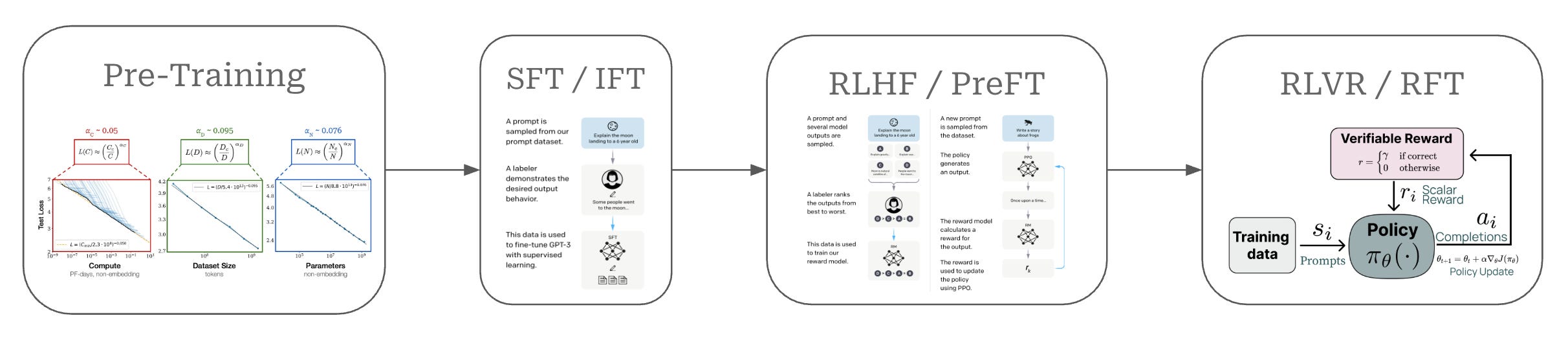
To begin, we will quickly delve into the role of alignment in LLM training and outline the many variants of online and offline alignment algorithms that currently exist. Modern LLMs are trained in several stages, as depicted in the figure above. The key training stages for an LLM are as follows:
Pretraining is a large-scale training procedure that trains the LLM from scratch over internet-scale text data using a next token prediction training objective; see here.
Supervised finetuning (SFT) or instruction finetuning (IFT) also uses a (supervised) next token prediction training objective to train the LLM over a smaller set of high-quality completions that it learns to emulate; see here.
Reinforcement learning from human feedback (RLHF) or preference finetuning (PreFT) uses reinforcement learning (RL) to train the LLM over human preference data; see here.
Reinforcement learning from verifiable rewards (RLVR) or reinforcement finetuning (RFT) trains the LLM with RL on verifiable tasks, where a reward can be derived deterministically from rules or heuristics.
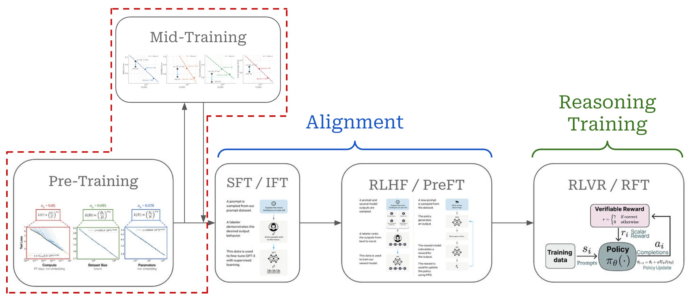
We can group the training strategies outlined above into distinct stages; see below. The pretraining (and midtraining) process focuses on building the core knowledge base of the LLM, while alignment teaches the LLM correct formatting and style for maximizing human preference scores. Reasoning training is a final step that yields an additional boost in performance on verifiable tasks.
This overview focuses on LLM alignment and the many algorithms—including SFT and many forms of RL-based and RL-free RLHF—that have been proposed. We will focus especially on the role and necessity of online RL—as opposed to using simpler, offline alignment algorithms—in the RLHF training process. In this section, we will kick off this discussion by explaining the many options that exist for alignment algorithms, including both online and offline algorithms.
Supervised Finetuning (SFT)
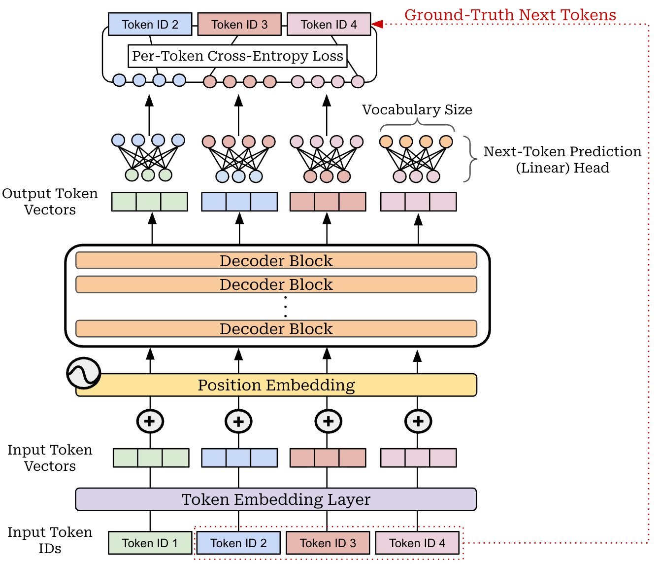
One of the simplest LLM alignment strategies is supervised finetuning (SFT), which adopts the same next token prediction training objective used during pretraining. We train the LLM to predict the next token in a sequence given all prior tokens as context (shown above)—this is a self-supervised training objective that can be applied efficiently to large volumes of raw text data. A basic implementation of the next token prediction training objective is provided below for reference.
import torch
import torch.nn.functional as F

# token_indices: (batch_size, seq_length)
logits = LLM(token_indices)  # (batch_size, seq_length, vocab_size)

# shift to predict next token at each position
logits = logits[:, :-1, :]  # (batch_size, seq_length - 1, vocab_size)
targets = token_indices[:, 1:]  # (batch_size, seq_length - 1)

# resize tensors for cross-entropy loss
logits = logits.reshape(-1, logits.size(-1))
targets = targets.reshape(-1)

# compute cross-entropy loss
loss = F.cross_entropy(logits, targets)
During pretraining, this training objective is applied over a massive corpus of text scraped from the internet. In contrast, SFT focuses upon curating a smaller set of high-quality prompt-response pairs for aligning the LLM. For example, LIMA is a popular paper that aligned an LLM using SFT with a curated dataset of only 1K examples. Recent LLMs use a larger number of samples in the SFT dataset; e.g., Tulu-3 is trained with ~1M SFT examples. Put simply, SFT aligns an LLM by training the model over concrete demonstrations of preferable responses.
In most cases, we can achieve better performance by using a completion-only loss in SFT, meaning that the cross-entropy loss is masked for all prompt tokens and only applied to tokens within the response or completion1. For a more detailed exposition of SFT, please see my prior overview on this topic linked below.
Understanding and Using Supervised Fine-Tuning (SFT) for Language Models

One of the most widely-used alignment techniques for LLMs is supervised fine-tuning (SFT), which trains the model over a curated dataset of high-quality demonstrations using a standard language modeling objective. SFT is simple / cheap to use and is a useful tool for aligning LLMs.
Rejection sampling is an online variant of SFT that is an extremely effective and easy to use. The standard formulation for SFT is offline—we train the model over a fixed dataset of prompt-response pairs. Rejection sampling changes this setup by:
Starting with a dataset of prompts.
Generating completions for each prompt with the current LLM.
Scoring all of these completions using a reward model or LLM judge.
Selecting (or filtering) the top-scoring prompt-completion pairs2.
Performing SFT over these top examples.
The rejection sampling process is depicted below. This approach trains the LLM in a similar fashion to SFT, but the difference lies in the data. We are using the LLM itself to sample SFT training data in a semi-online fashion. The reward model is used to ensure that we are training over the highest-quality completions.

We typically perform rejection sampling iteratively. For example, the Llama-2 alignment process uses four rounds of rejection sampling before RL-based RLHF.
In the discussion above, we described rejection sampling as a variant of SFT, since both use the same training objective. However, rejection sampling is actually a preference tuning technique and is most often used as a simpler alternative to RLHF—not as an alternative to SFT. In practice, rejection sampling is usually applied after SFT, rather than in place of it.
SFT variants. Beyond rejection sampling (also called Best-of-N sampling), there are several online or iterative variants of SFT that have been proposed. Some notable examples that we will encounter in this overview include:
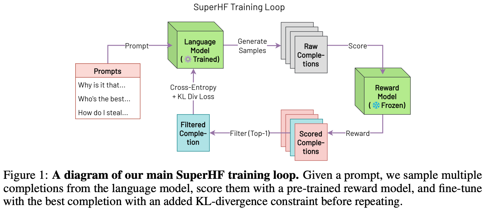
Supervised Iterative Learning from Human Feedback (SuperHF) [13] is an online learning technique that samples a batch of on-policy outputs from a model, filters these outputs with a reward model, and optimizes the model using a supervised objective under a KL divergence constraint; see above.
Reinforced Self-Training (ReST) [14] uses the rejection sampling formulation outlined above, in which we iteratively sample on-policy data from the LLM, score each sample with a reward model, and train on the best samples.
Reward-Weighted Regression (RWR) [15] similarly uses the LLM to generate on-policy samples that are scored with a reward model. But, these scores are used to weight each sample in the training loss instead of for filtering.
Reward Ranked Finetuning (RAFT) [16] again adopts the standard rejection sampling setup that samples online completions from the LLM and filters these completions for use in SFT with scores from a reward model.
Reinforcement Learning (RL) Training

There are two different types of reinforcement learning (RL) training that are commonly used to train LLMs (shown above):
Reinforcement Learning from Human Feedback (RLHF) trains the LLM using RL with rewards derived from a human preference reward model.
Reinforcement Learning with Verifiable Rewards (RLVR) trains the LLM using RL with rewards derived from rules-based or deterministic verifiers.
These RL training techniques differ mainly in how they derive the reward for training, but other details of the algorithms are mostly similar. As depicted below, they both operate by generating completions over a set of prompts, computing the reward for these completions, and using the rewards to derive a policy update—or an update to the LLM’s parameters—with an RL optimizer.
![[animate output image]](https://substackcdn.com/image/fetch/$s_!uPv8!,f_auto,q_auto:good,fl_progressive:steep/https%3A%2F%2Fsubstack-post-media.s3.amazonaws.com%2Fpublic%2Fimages%2F56eba05c-359c-400d-920f-38a36dd4690a_1920x1078.gif "[animate output image]")
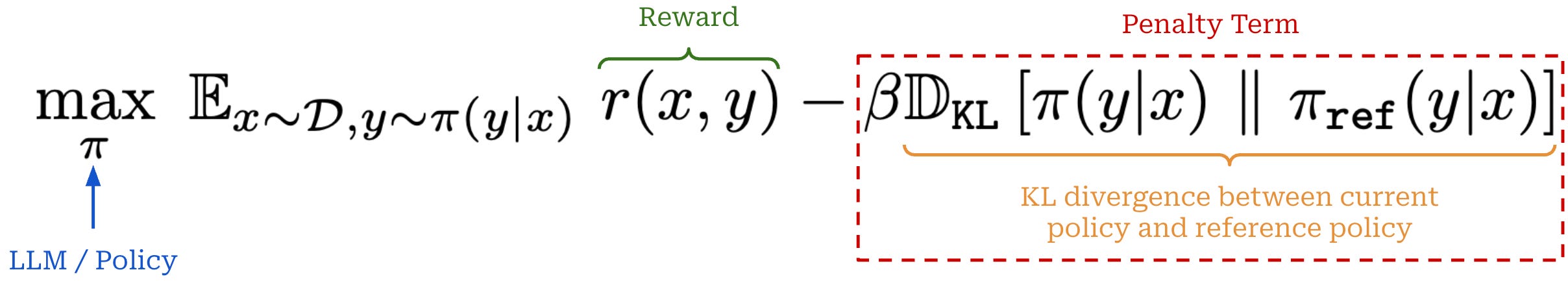
When we are optimizing an LLM with RL, we are trying to solve the objective shown below. This objective maximizes the reward received by the LLM’s completions while minimizing the KL divergence of the model with respect to a reference model—usually an LLM checkpoint from the start of RL training. Put simply, this means that we want to maximize reward without making our new model significantly different from the original (reference) model.
On-policy sampling. As shown above, we perform on-policy sampling when training an LLM with RL. By “on-policy” sampling, we mean that completions used to train our LLM in the core RL training loop are generated in real-time by the LLM itself—the completions are not generated by another model or stored in an offline, pre-computed dataset. In the context of LLMs, training algorithms that use on-policy sampling are typically referred to as “online” training algorithms. On-policy sampling is not only used within the context of RL training; e.g., we learned about several online variants of SFT in the prior section.
More on RLHF. This overview is focused upon LLM alignment, so we will mostly encounter RLHF-style training. Early approaches to LLM alignment used the three-stage technique (shown below) that combines SFT with RLHF.

In RLHF, we begin by collecting a dataset of preference pairs, where each preference pair contains:
A prompt.
A chosen (or winning) completion.
A rejected (or losing) completion.
We then train a reward model over the preference dataset and optimize our LLM with the RL training loop described above. The completions in this preference dataset can come from a variety of sources; e.g., the reference model, prior model checkpoints, or even completely different models. The preference annotation—or selection of the chosen and rejected completion in the pair—is usually provided either by a human annotator or LLM judge (i.e., AI feedback). Notably, the preference data and reward model are fixed at the beginning of RL training. Making this a bit more formal, LLMs are trained with a variant of offline model-based RL.
RL optimizers. There is one detail missing from the above explanation of RL training: how do we compute the policy update? We will briefly address this question here, but interested readers should see this in-depth overview for full details. Usually, a policy gradient-based RL optimizer (e.g., REINFORCE, PPO, or GRPO) is used. PPO-based RLHF has been the de facto choice in the past, but PPO is computationally expensive due to estimating the value function with an LLM. In fact, PPO-based RLHF stores four different copies of the LLM during training (i.e., the policy, reference policy, value model, and reward model).
To reduce overhead, REINFORCE derives a monte carlo estimate of the policy gradient by approximating the value function with an average of rewards received by the model throughout training (i.e., instead of with an LLM). In a similar vein, GRPO approximates the value function with an average of rewards from multiple completions to the same prompt—referred to as a group. Because GRPO is the most common RL optimizer for RLVR, it is also commonly used without a reward model. In this case, we only store two copies of the LLM—the policy and reference policy—for RL training. However, the lack of a reward model is a byproduct of RLVR (i.e., GRPO can be used with or without a reward model).
Direct Alignment Techniques
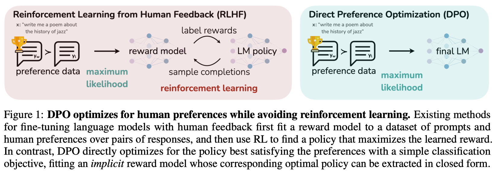
Because online RL training is so expensive, researchers have also proposed offline alignment techniques like direct preference optimization (DPO) [18]. Compared to PPO-based RLHF, DPO avoids training an explicit reward model and instead derives a reward signal implicitly from the LLM itself. Using this implicit reward, the LLM is trained with the contrastive learning objective shown below, which can be optimized using standard gradient descent (i.e., without any RL training).

Intuitively, this contrastive loss increases the probability margin between chosen and rejected responses in a preference dataset. The LLM is trained on a fixed preference dataset—the same data that is used to train the reward model in RLHF. For this reason, DPO is characterized as an offline—meaning the training data is fixed and there is no on-policy sampling—direct alignment algorithm. Compared to RL-based alignment algorithms, DPO requires much less computational overhead, is easier to tune, and still tends to perform well; see below for more details.
Direct Preference Optimization (DPO)

Alignment techniques like RLHF led to massive improvements in LLM quality, but they are computationally expensive and hard to use. This overview covers a simpler approach to LLM alignment, called DPO, that avoids these complexities by aligning LLMs with an objective that can be optimized with gradient descent.
Variants of DPO. Because DPO was so much simpler to use relative to PPO-based RLHF, this technique quickly became popular within LLM research. As a result, many variants of DPO were proposed, such as Identity Preference Optimization (IPO) [8], Kahneman-Tversky Optimization (KTO) [19], or Contrastive Preference Optimization (CPO) [20]. Many of these techniques make slight modifications to DPO that yield a mild boost in performance, but the core idea behind them—in terms of using direct alignment with a contrastive objective—is similar. Some of these techniques, however, are meaningfully different from DPO; e.g., KTO formulates a DPO-style loss than can be applied to a single completion with a binary (good or bad) rating as opposed to a preference pair.
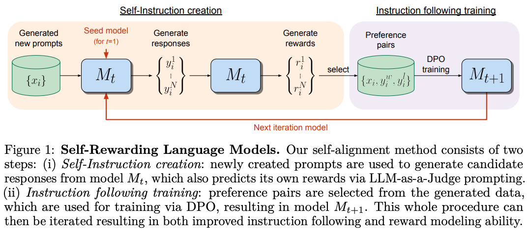
Online or iterative DPO. In its standard formulation, DPO is a completely offline alignment algorithm. The preference dataset is fixed throughout DPO training, but we can create online (or semi-online) DPO variants by introducing on-policy samples into the training process. As depicted below, one example of this idea is self-rewarding language models [10]. In this framework, we periodically sample fresh data for DPO training as follows:
Start with a set of prompts.
Sample multiple completions to these prompts with the current LLM.
Rank these completions (e.g., using an LLM judge or a reward model) to create a preference dataset.
Train the LLM over this data using DPO.
Return to step one and repeat for several rounds.
In this process, we iteratively train the model with DPO, but the training data is periodically re-sampled from the current policy—this is a semi-online training setup. We can make this approach more on-policy by sampling completions from the current policy more regularly. In fact, we can even create a fully-online DPO variant by sampling on-policy completions for every batch of training data!
The Online-Offline Performance Gap
Although PPO-based RLHF was the standard choice for LLM alignment for some time, this approach is expensive, complex, and difficult to replicate outside of top LLM labs. As a result, researchers have developed a variety of simpler alignment algorithms based on offline and RL-free training strategies. In this section, we aim to answer the following question: Does using offline alignment techniques come at a cost in performance? To address this, we will review a range of papers that study the impact of offline training, the use of on-policy samples, contrastive training objectives, and other factors on LLM performance.
Is DPO Superior to PPO for LLM Alignment? A Comprehensive Study [6]
“Experiment results demonstrate that PPO is able to surpass other alignment methods in all… Particularly, in the most challenging code competition tasks, PPO achieves state-of-the-art results.” - from [6]
We see several different avenues of comparing PPO-based RLHF and (offline) DPO in [6], including theoretical analysis, synthetic experiments and practical training of LLMs. The goal of this work is to find and explain the limitations of DPO in LLM alignment. First, authors confirm there is a performance gap between DPO and PPO-based RLHF. Then, they provide analysis that uncovers the key reason for this trend—the performance of DPO is significantly impacted by the presence of out-of-distribution examples in its underlying preference dataset.
Reward hacking. When training an LLM with PPO-based RLHF, we generate completions to prompts in our prompt dataset in an online fashion and score them with a reward model. Given that our reward model is an LLM that is trained over a fixed (and biased) preference dataset, this model is an imperfect proxy for the actual, ground-truth reward—it can make mistakes in the scores that it provides! Going further, the LLM being trained by PPO can also learn to exploit these mistakes by finding a way to erroneously maximize rewards provided by the reward model without actually meeting human preference expectations.
This phenomenon—commonly referred to as “reward hacking”—has a long history of study within the RL literature. However, we see in [6] that similar issues can occur even when using RL-free, offline alignment algorithms like DPO. In particular, authors make the statement quoted below, which tells us that:
Any solution found by PPO also minimizes the training objective for DPO (i.e., the set of solutions to PPO is a subset of the solutions to DPO).
It is possible for PPO to find erroneous (or reward-hacked) solutions.
Therefore, the same erroneous solutions can also be discovered with DPO.
Given a ground-truth reward r and a preference dataset D, let Π_PPO be the class of policies induced by training reward model R_Φ over D and running PPO. Let Π_DPO be the class of policies induced by running DPO. We have the following conclusion: Π_PPO is a proper subset of Π_DPO. - from [6]
Due to not using an explicit reward model, DPO cannot be reward hacked in a similar manner to PPO. However, DPO still suffers from similar issues with out-of-distribution data in a different manner. Specifically, DPO learns a bias towards unseen—or out-of-distribution—completions as explained below.
“DPO can develop a biased distribution favoring unseen responses, directly impacting quality of the learned policy… DPO is prone to generating a biased policy that favors out-of-distribution responses, leading to unpredictable behaviors.” - from [6]
This bias is most pronounced when there is a large distribution shift between the reference model used in DPO and the model used to generate completions within the preference dataset. Ideally, these completions should be generated with the reference model used in DPO. While online algorithms like PPO generate on-policy completions during training, offline algorithms like DPO are trained over a fixed preference dataset, where completions can come from an arbitrary LLM.
Synthetic example. To validate DPO’s issues with out-of-distribution data, a simple synthetic training example is constructed in [6]. In this setup, the policy is a basic multi-layer perceptron that takes a one-hot vector as input (i.e., the prompt) and produces an eight-dimensional categorical distribution as output3. We assume that the optimal policy is diagonal as illustrated in the plots below.
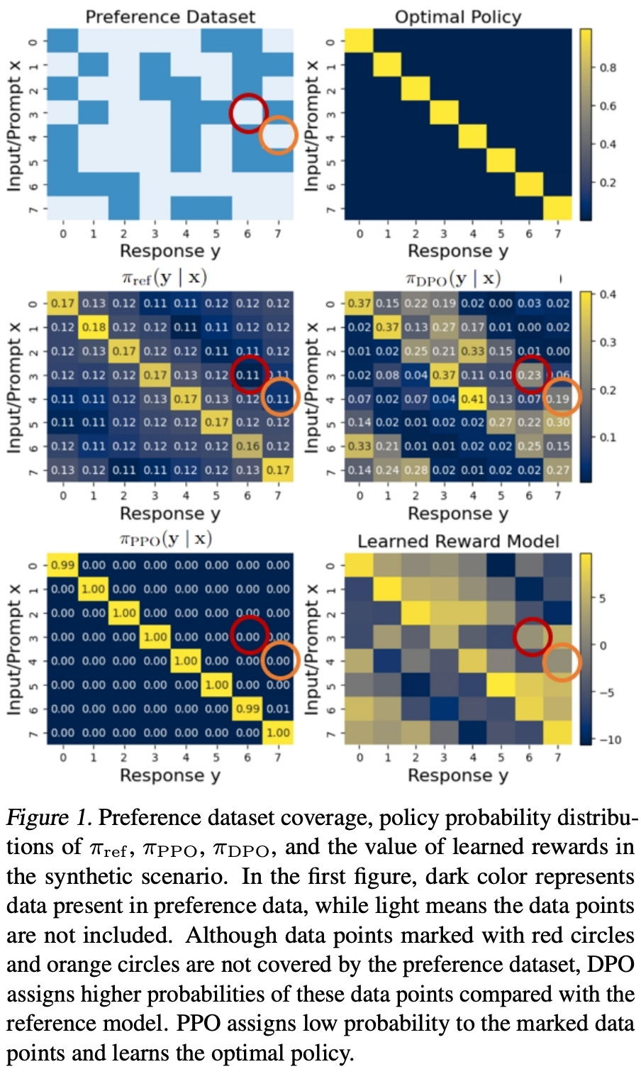
Using this toy setup, we can create synthetic preference datasets that purposely omit certain preference pairs from the training data, thus testing the behavior of both DPO and PPO in handling out-of-distribution data. As shown above, PPO handles this coverage issue correctly and recovers the optimal policy. In contrast, DPO incorrectly learns to assign high probability to data that is out-of-distribution, which validates—at least at a small scale—the argument in [6] that DPO develops an erroneous bias towards out-of-distribution data in the preference dataset.
Practical experiments. Following this synthetic test, larger-scale preference tuning experiments are performed with various Llama-2-derived LLMs on the SafeRLHF dataset. Experiments begin with an SFT model trained on the Alpaca dataset, creating a distribution shift between the SFT model and the preference data—completions in the Alpaca dataset are much different than those of SafeRLHF.
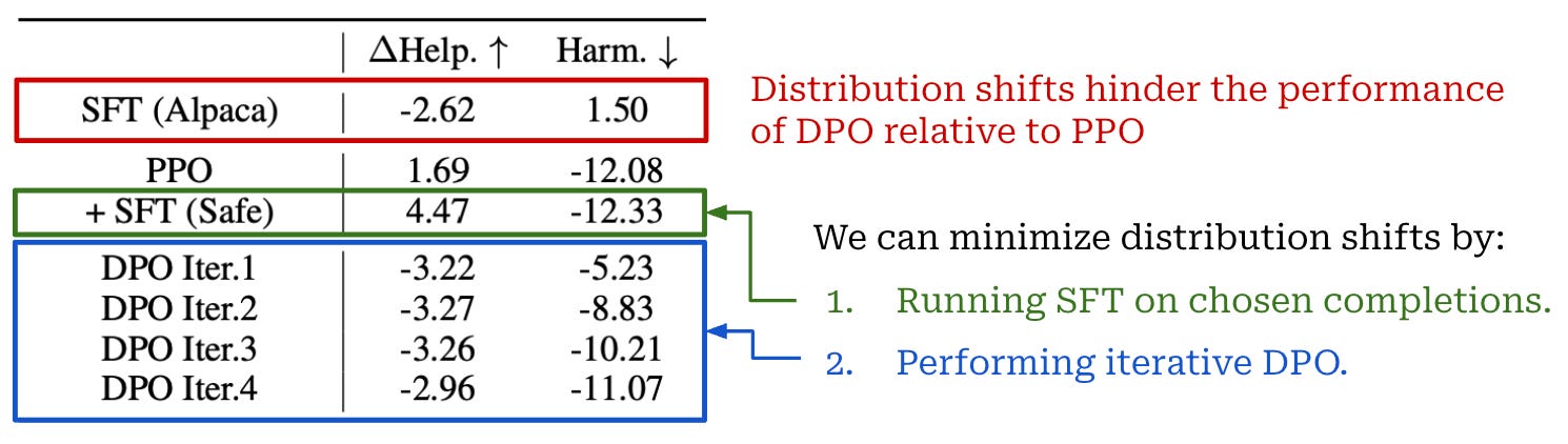
As shown above, using the Alpaca SFT model directly as the starting point for DPO performs poorly, but performance improves drastically when we first finetune the Alpaca SFT model over preferred completions in the SafeRLHF dataset prior to performing DPO training. These results indicate that a distribution shift between the reference model and preference data in DPO is indeed detrimental to LLM performance in practical alignment scenarios. Notably, the approach of running additional SFT over preferred completions in the preference dataset prior to DPO was also recommended in the original DPO paper [1]!
“We generate new responses with SFT (Safe) and use a learned reward model for preference labeling. We further repeat this process and iteratively set the reference model as the latest DPO model in the last iteration.” - from [6]
A new approach for avoiding out-of-distribution data via iterative DPO is also proposed in [6]. We can run several rounds of DPO, where at each round we use the current reference policy to generate fresh completions that are automatically scored by reward model to create a preference dataset. After each round, our current policy becomes the new reference policy, and we repeat this process, thus ensuring there is no distribution shift between our reference policy and the preference dataset. Using this approach, we can train a model with comparable safety (but not helpfulness) ratings to those obtained with PPO, thus narrowing the performance gap between online and offline alignment algorithms.
Preference Fine-Tuning of LLMs Should Leverage Suboptimal, On-Policy Data [7]
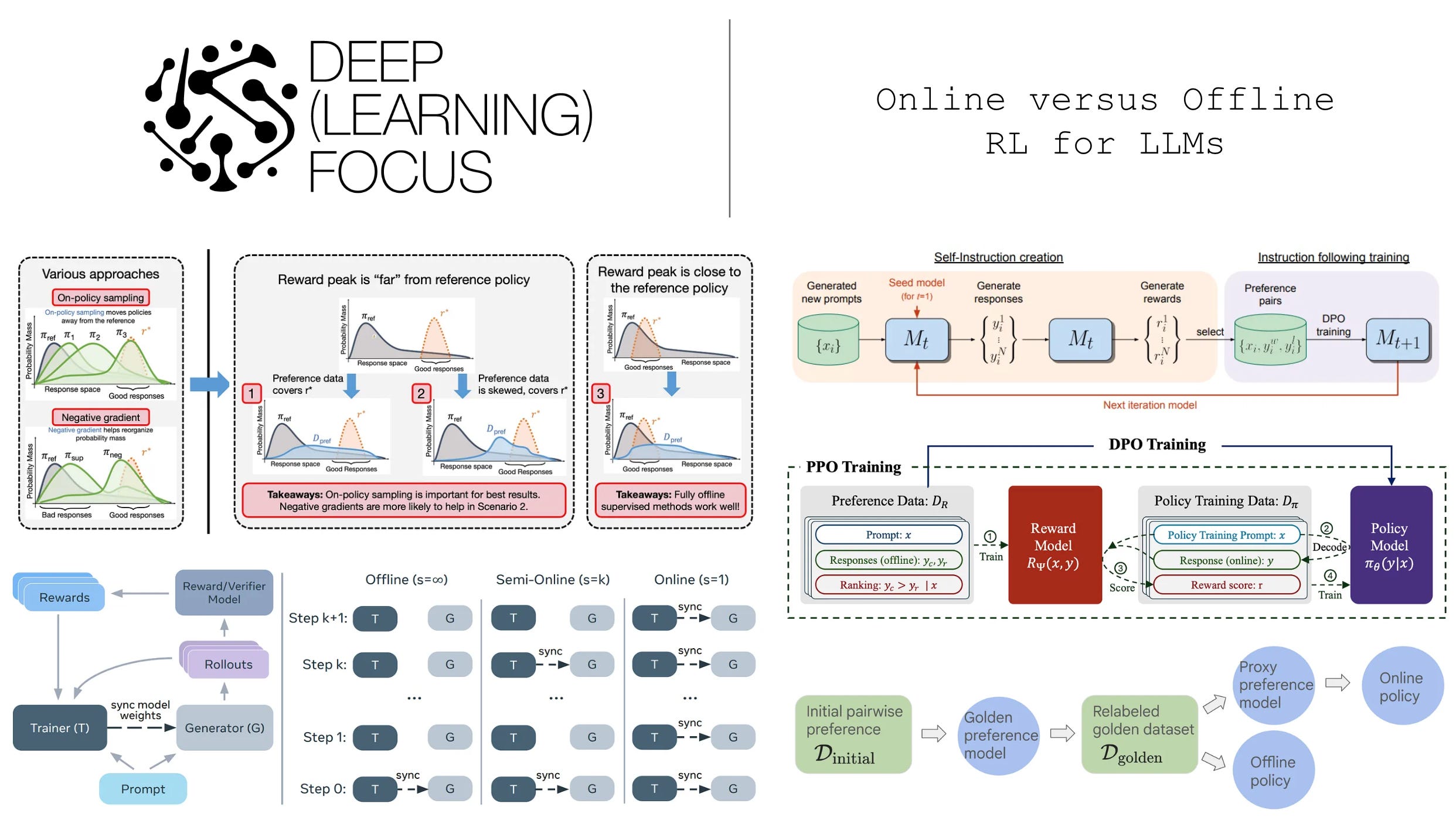
By conducting a comprehensive study that covers nearly every possible alignment strategy for an LLM, authors in [7] discover two key characteristics that create a successful alignment algorithm:
The use of on-policy sampling.
The presence of a “negative gradient” that decreases probability of bad responses; i.e., instead of only increasing the probability of good responses.
For example, SFT purely trains the LLM using a maximum likelihood objective over a set of high-quality completions, while DPO leverages a contrastive objective that both i) increases the probability of the chosen response and ii) decreases the probability of the rejected response. However, the training data is fixed for both of these strategies—they perform no on-policy sampling. We can fix these issues by using an online RL algorithm like PPO or adopting an iterative DPO strategy that periodically samples new data from the current policy.
“Our main finding is that, in general, approaches that use on-policy sampling or attempt to push down the likelihood on certain responses outperform offline and maximum likelihood objectives.” - from [7]
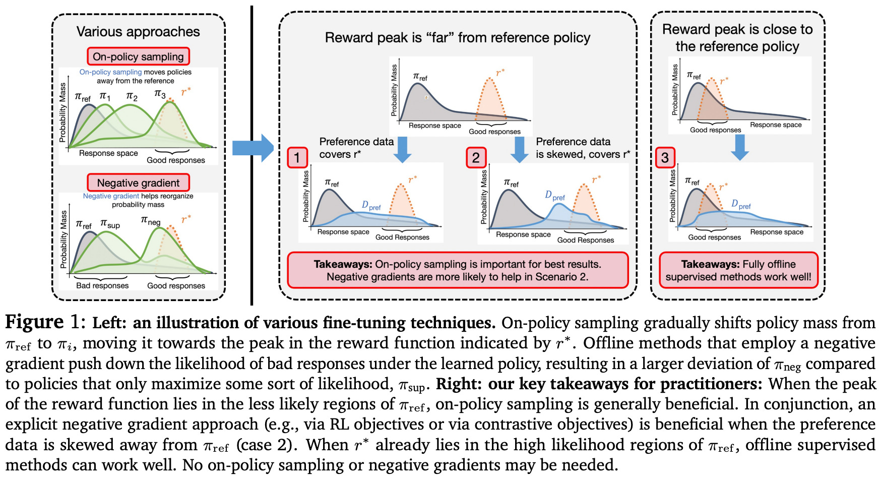
We also learn in [7] that on-policy sampling and negative gradients are most useful in difficult alignment cases, where the responses that receive high rewards are unlikely within the reference policy. In such cases, the alignment process must train the LLM by “moving” probability mass away from low-reward responses and toward high-reward responses. Offline and purely supervised alignment methods perform especially poor in these complex scenarios.
Alignment algorithms. Authors in [5] begin by characterizing a wide set of potential alignment algorithms (shown below) based on their use of on-policy sampling, negative gradients, and sample reuse (i.e., performing multiple gradient updates over the same data). As a concrete example of sample reuse, PPO executes two to four sequential gradient updates over each batch of training data, while GRPO4 and REINFORCE typically avoid such sample reuse [9].
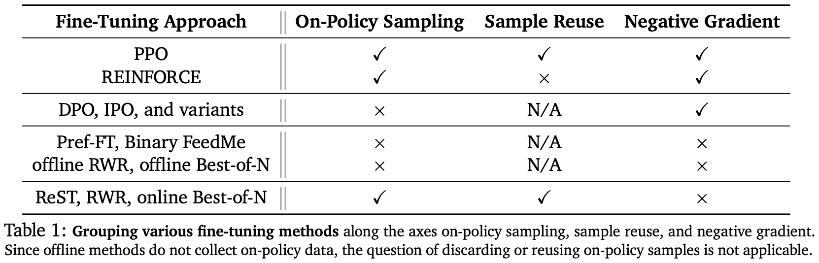
All SFT and rejection sampling variants lack the negative gradient that is present in RL-based and direct alignment methods, where we explicitly decrease the probability of responses that are either rejected (for direct alignment) or receive a low reward (for RL). Finally, on-policy sampling may or may not be used by most techniques depending on the training setup. Direct alignment methods like DPO or IPO run contrastive training on a fixed preference dataset with no on-policy sampling, but we can create an online version of an offline algorithm by periodically sampling new training data from the current policy. However, some algorithms like PPO and REINFORCE are naturally based upon on-policy sampling.
Unified alignment algorithm. To capture the scope of possible alignment algorithms, authors in [7] create the framework shown below. This framework enables the systematic study of different settings within the underlying alignment algorithm. For example, steps one and two can be performed either:
With on-policy data collection (i.e., by generating responses from the current policy and automatically scoring them with a reward model).
By directly using offline preference data without any on-policy sampling (e.g., as in standard DPO).
Going further, we can vary the extent of on-policy sampling by changing the total number of samples B or varying total gradient steps T performed on a set of samples. Notably, increasing T introduces sample reuse while increasing B does not, thus allowing us to isolate the impact of reusing on-policy samples.
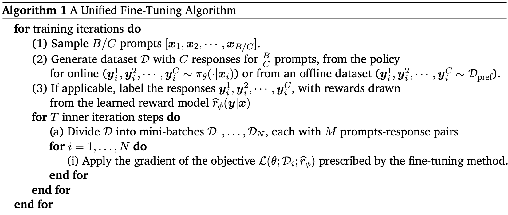
Notably, this unified algorithm does not capture any of the maximum likelihood alignment algorithms, though these algorithms are still considered in [7].
Training setup. The properties of these different alignment algorithms are analyzed using several experimental setups including:
Small-scale (didactic) bandit problems.
Synthetic LLM problems.
Full-scale LLM alignment.
In the synthetic alignment scenario, we use hand-crafted rewards based on the length of the LLM’s response. Specifically, two reward settings are considered—minimizing the response length and matching the average response length; see below. These reward scenarios test cases in which high-reward responses lie both within and outside of the region of probable completions for the reference policy5.
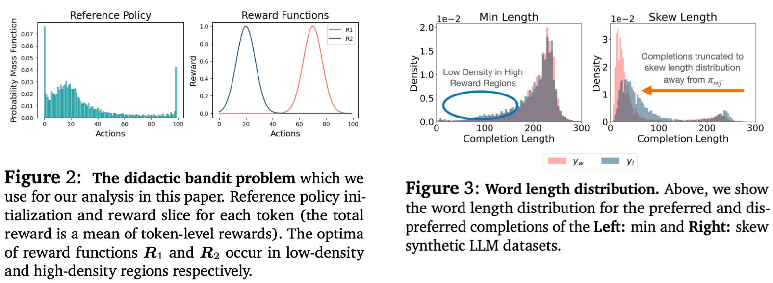
The didactic bandit problems also test multiple reward setups that change the optimum of the reward function. By changing the reward setup, we test each algorithm’s ability to assign probability to high-reward responses, even if these responses have low probability in the original reference policy; see above.
“The optimum of the reward function R1 is located in low likelihood regions of the reference policy, whereas the optimum of R2 is roughly aligned with the mode of the reference policy. We hypothesize that on-policy sampling will be crucial to optimize reward function R1, whereas offline or maximum likelihood methods could be sufficient for the optimization of R2.” - Bandit problem description from [7]
The full-scale alignment scenario uses public preference data from AlpacaFarm, UltraChat and UltraFeedback to align smaller-scale LLMs like Pythia-1.4B and Mistral-7B. This training setup is a more standard LLM alignment scenario, and models are evaluated using a golden human preference reward model.
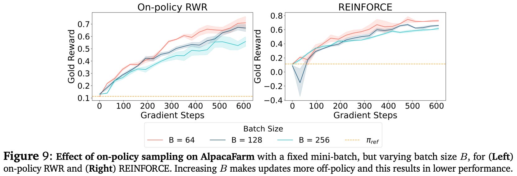
The role of on-policy sampling. We learn from experiments in [7] that sampling on-policy data more frequently and in smaller batches—the most strictly on-policy setup possible—leads to the best performance. The impact of on-policy sampling is most noticeable in complex alignment scenarios, where high-reward responses do not already lie within the probable region of the reference policy.
“[We] observe strong and clear trends supporting that on-policy sampling with a smaller but frequently sampled batch results in better performance… The performance degradation with more off-policy updates is substantially milder for 𝑅2, indicating that when the peak in the reward function lies in the likely regions of the reference policy, a higher degree of off-policy updates is tolerable.” - from [7]
In simper alignment cases where responses that receive high rewards are already probable within the reference policy, the model can better tolerate the use of offline training algorithms. This phenomenon is confirmed in both synthetic and didactic problem setups. Additionally, we observe the same trend in full-scale LLM alignment experiments, where the highest reward comes from decreasing the batch size B to make the training process more on-policy; see below.
The negative gradient. Similarly to on-policy sampling, the use of a negative gradient is found to benefit alignment. Algorithms that employ a negative gradient have a noticeable boost in performance relative to those that do not, especially in difficult alignment cases where we must increase the probability of responses that were originally assigned low probability by the reference policy. As shown below (top figure), algorithms that employ a negative gradient increase the probability margin between chosen and rejected responses during training. Such a trend is not observed for algorithms that lack a negative gradient.
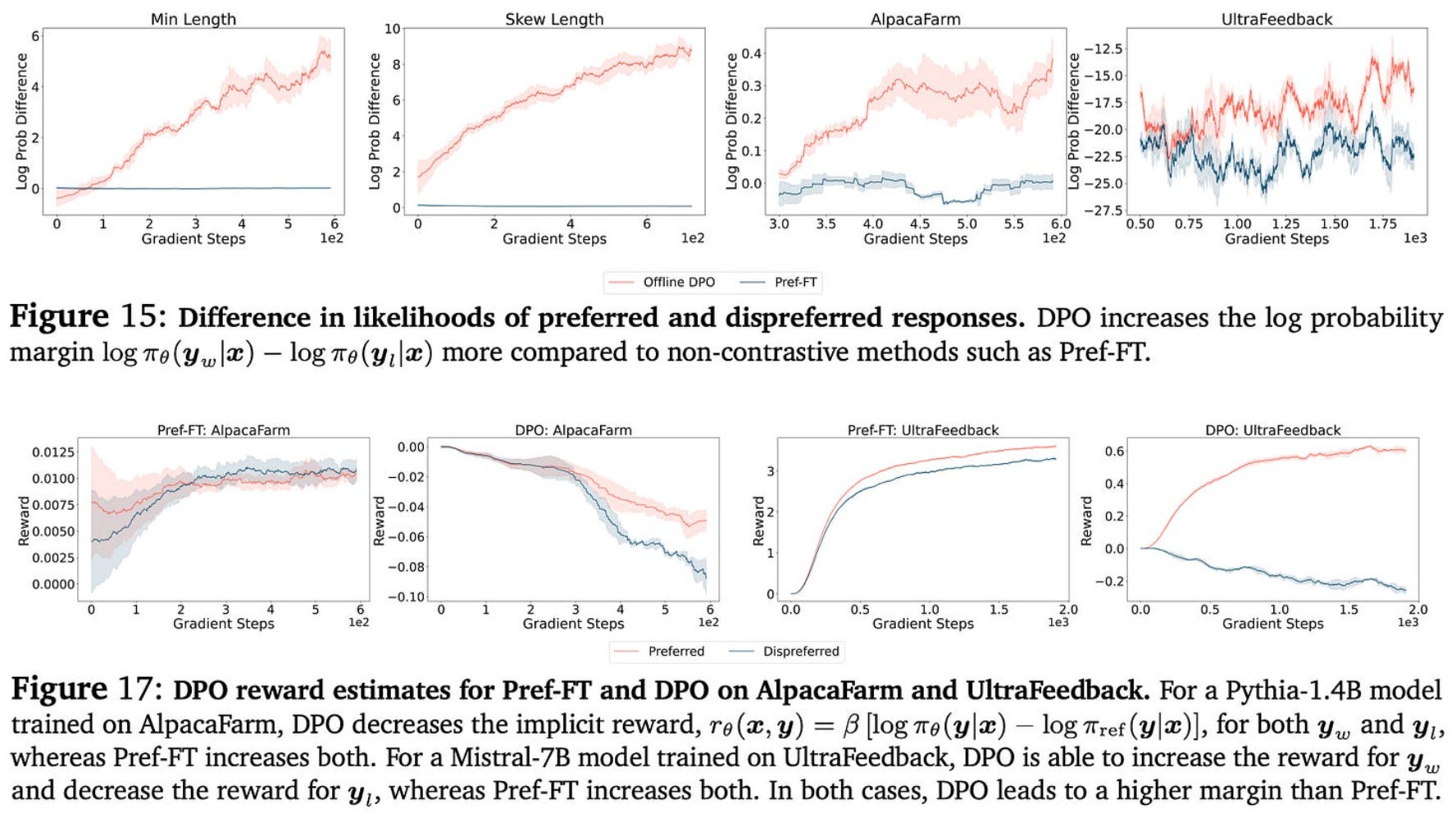
Interestingly, however, we see above (bottom plot) that the absolute probability of both chosen and rejected responses actually decreases during training despite an increasing margin. This same trend has also been observed in other papers [8].
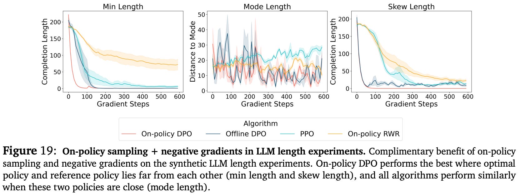
On-policy sampling and negative gradients yield compounding benefits when used in tandem. For example, on-policy IPO and DPO have faster convergence and better performance compared to offline variants in both didactic bandit and synthetic LLM experiments; see above. In full-scale LLM experiments, online versions of contrastive alignment algorithms outperform PPO in some cases despite having lower computational costs and wall-clock training time.
Is sample reuse detrimental? Substantially increasing the value of T would trivially degrade performance due to the introduction of off-policy data into the training process. However, moderate settings of T could allow the model to incorporate off-policy updates into the training process without causing a large drop in performance. For example, the synthetic LLM setting with PPO has no noticeable degradation in performance when increasing T from 1 to 8; see below.
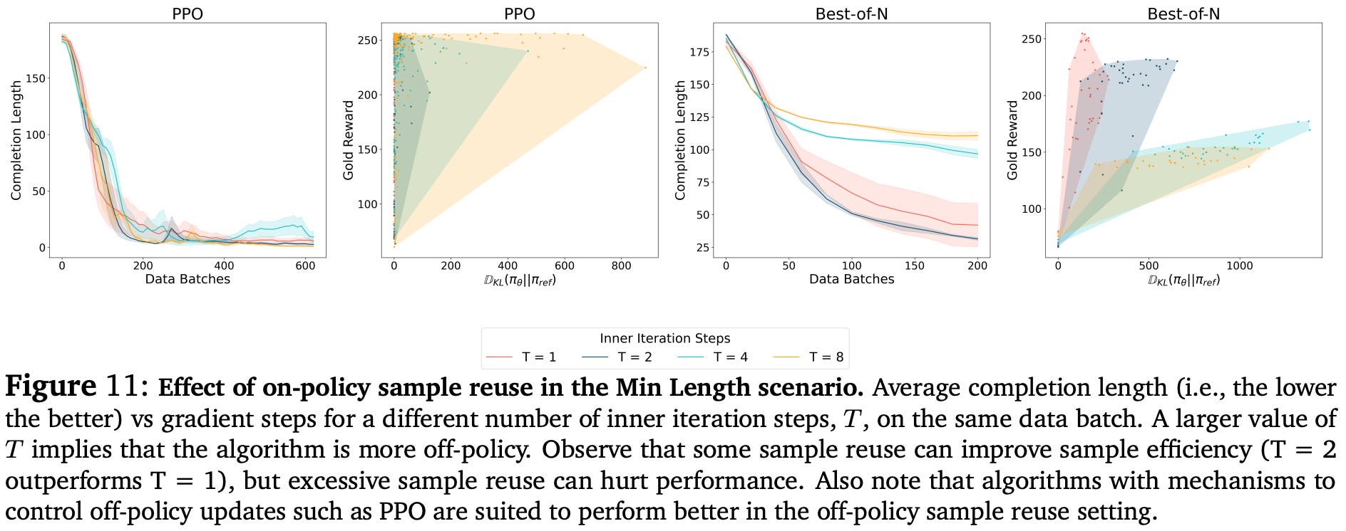
Maximum likelihood training objectives like rejection sampling (called Best-of-N in the figure above) are more sensitive to sample reuse6 but can still achieve good results with more moderate settings of T. Put simply, these results show that off-policy updates from sample reuse do not seem to hurt an LLM’s performance.
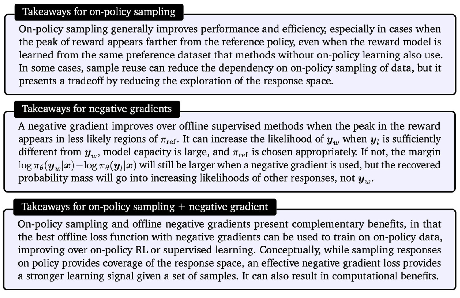
The key takeaways from alignment experiments in [7] are depicted in the figure above and can be summarized as follows:
On-policy sampling is crucial for high-quality alignment, especially if responses with optimal reward are not likely in the reference policy.
Moderate amounts of sample reuse can introduce off-policy updates without causing a noticeable deterioration in alignment quality.
The use of negative gradients leads to faster convergence and has a complementary benefit to on-policy sampling.
For simple alignment cases where the peak in rewards is already likely in the reference policy, fully offline or supervised methods—which use no on-policy sampling or negative gradient—can still perform well.
Each of these key points are also captured by the practical alignment takeaways presented in [7], which have been copied below for easier reference.
Unpacking DPO and PPO: Disentangling Best Practices for Learning from Preference Feedback [2]
In [2], authors perform an empirical comparison between online and offline RL algorithms—PPO-based RLHF and DPO in particular—for aligning medium-scale LLMs. This analysis tries to maximize the performance of a single LLM across a wide set of benchmarks spanning several domains by varying:
The type, source or scale of preference data being used.
The style of training algorithm (i.e., offline or online).
Additionally, several hyperparameter settings and training setups are considered for improving the performance of PPO-based RLHF, providing useful intuition for maximizing results with online RL. From this analysis, we learn that:
The choice of preference data has the greatest impact on LLM quality—data quality and composition are the key determinants of success in alignment.
Online RL algorithms consistently outperform offline algorithms like DPO.
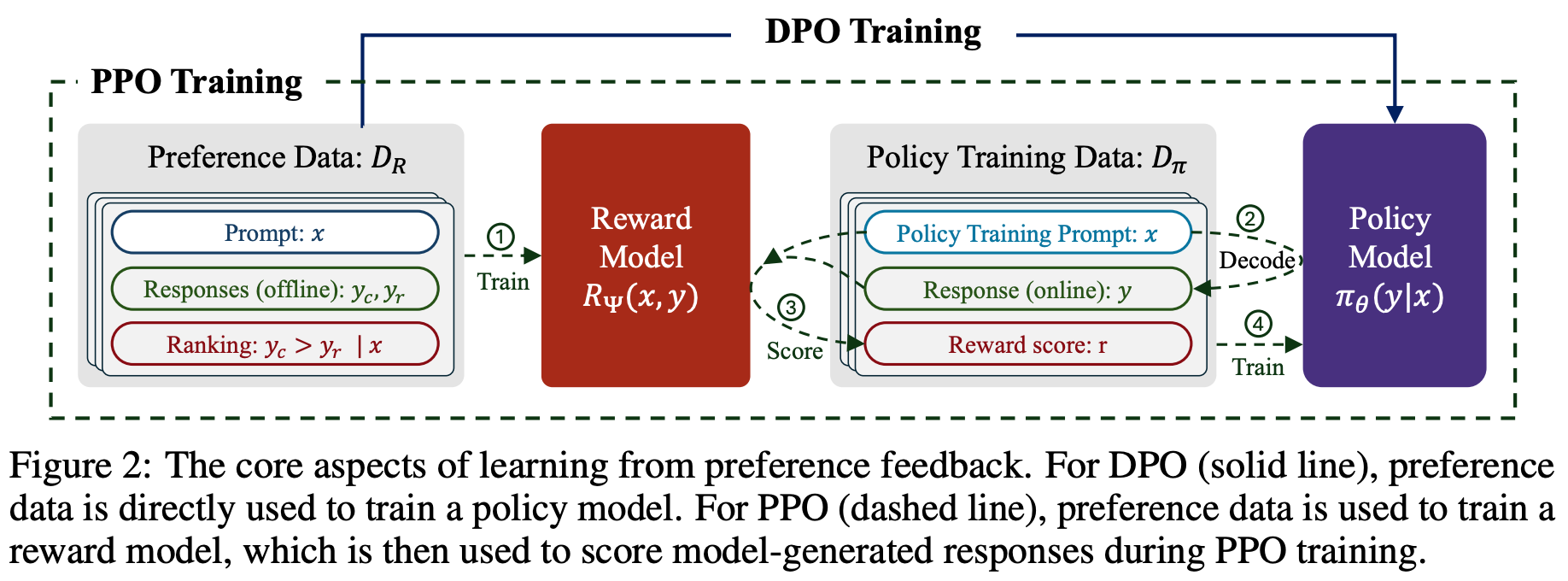
The experimental setup in [2] adopts a standard approach for both PPO-based RLHF and DPO; see above. All experiments use Tulu-2-13B [3] as the starting model for both DPO and PPO. After preference tuning, models are evaluated over a wide set of benchmarks that measure performance in the following domains:
Factuality (e.g., MMLU)
Reasoning (e.g., GSM8K)
Truthfulness (e.g., TruthfulQA)
Coding (e.g., HumanEval+)
Safety (e.g., ToxiGen)
Instruction following (e.g., IFEval)
From these diverse benchmarks, we can observe the performance of models in individual domains, as well as their general performance across domains.
Data selection. Building upon recent work that leverages synthetic preferences for LLM alignment [4], we can derive preference data from three sources:
Human preferences.
Web scraping7.
Synthetic preferences.
Interestingly, we learn in [2] that synthetic preference datasets—and the UltraFeedback dataset in particular—yield the best results, even compared to human-annotated preference data. Going further, authors in [2] specifically mention the following important considerations for curating preference data:
The quality of preferences (i.e., the choice of chosen or rejected completion within a preference pair) is actually more important than the quality of the completions themselves.
Collecting per-aspect preference feedback yields a clear performance benefit—models trained on aggregated, per-aspect preferences outperform those trained on
15xthe amount of standard preference data.With the data that was considered in [1], preference tuning has the biggest impact on improving chat capabilities and output style, but the model does not seem to learn new facts or information.
Per-aspect preference feedback is collected by asking a human or model to score each aspect of the data (e.g., helpfulness and harmlessness) independently, then aggregating these per-aspect scores to yield a final, aggregated preference score. Compared to just asking annotators for a single overall preference score, such an approach is found to improve the quality of preference feedback, which in turn improves the quality of resulting models after preference tuning. Authors in [2] consider various factors that impact the quality of post-training, but the source and quality of preference data are found to have the most significant impact.
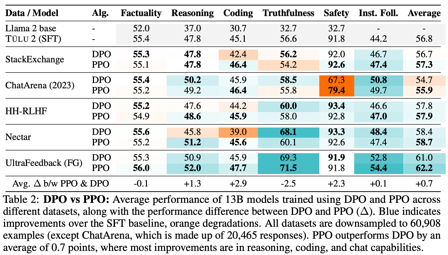
“PPO outperforms DPO by up to 2.5% in math and 1.2% in general domains. High-quality preference data leads to improvements of up to 8% in instruction following and truthfulness.” - from [2]
PPO vs. DPO. When directly comparing models trained with an online or offline approach, we see in [2] that online training algorithms have a clear edge. In fact, nearly all models trained with PPO-based RLHF across all datasets are found to outperform those trained with DPO using identical settings. Results in [1] provide clear evidence that online RL benefits preference tuning for LLMs; see below.
Why is online training so beneficial? The answer to this questions is complex and multi-faceted, but authors in [2] make an interesting observation regarding the difference between models trained with DPO and PPO. Namely, PPO models are far more likely to perform chain-of-thought reasoning for solving complex problems, even without being provided any examples of this behavior.
“Models trained with PPO are far more likely than DPO-trained models to perform chain-of-thought reasoning… even when not given in-context examples using chain-of-thought. This suggests that reasoning improvements from PPO may be due to increased chain-of-thought abilities.” - from [2]
Such behavior would be impossible for an LLM to learn with offline algorithms like DPO, as the completions from which the model learns are fixed within the preference dataset. On the other hand, PPO is able to learn such new behaviors because completions are sampled online during training, allowing the model to explore—and learn from—new behaviors like chain-of-though reasoning.
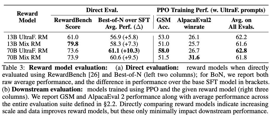
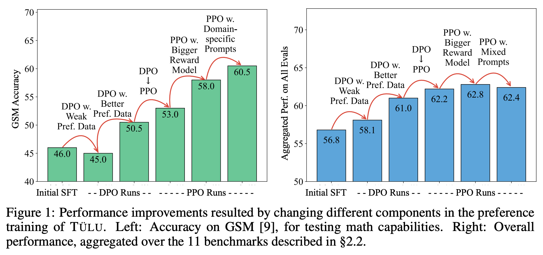
Other factors in online RL. Beyond the analysis of offline and online algorithms in [2], authors perform various other ablations to determine key factors to success in PPO-based RLHF. For example, increasing the size of the reward model—and the size of the preference dataset over which the reward model is trained—is found to improve the quality of the reward model. However, the impact of a better reward model on downstream evaluation benchmarks (i.e., after training the LLM with PPO-based RLHF) is less clear. The main performance benefits are observed in more complex domains like reasoning. Seemingly, a more powerful reward model is only impactful in challenging domains that actually require a better reward model.
“If we’re using a bigger reward model, we need to have data that is actually challenging the reward model.” - source
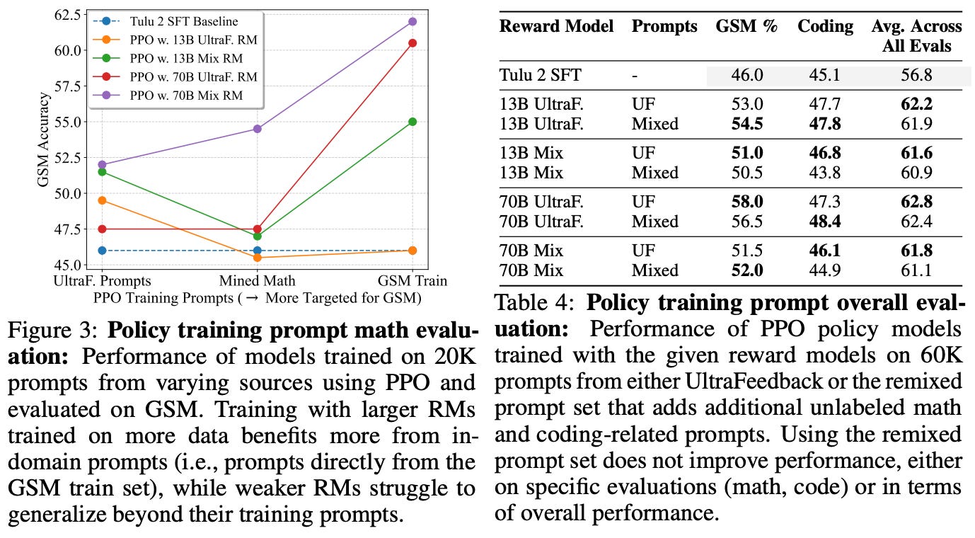
We can also boost the performance of the LLM in specific domains by curating a targeted prompt dataset for PPO that focuses on that domain—this is a unique benefit that can be exploited by PPO but is not possible in offline algorithms like DPO. However, such an approach does not yield performance improvements in general—it is only useful for tailoring the LLM to specific domains like math; see below.
The best training recipe. To conclude their analysis, authors in [2] emphasize the following aspects of LLM alignment:
The importance of preference data quality.
The superiority of online RL.
The benefit of better reward models in complex domains like reasoning.
The ability of targeted prompt datasets for PPO to curate an LLM’s performance to a particular domain.
The optimal approach for performing LLM alignment—as discovered by experiments performed in [2]—is summarized by the quote below.
“We take a high-quality, synthetic preference dataset, a large reward model, and train it using PPO. If we additionally wish to focus on a specific domain, we can additionally collect domain-specific prompts for policy training.” - from [2]
Understanding the performance gap between online and offline alignment algorithms [5]
“We show that on a suite of open source datasets, online algorithms generally outperform offline algorithms at the same optimization budget of KL divergence against the SFT policy” - from [5]
Authors in [5] analyze the importance of on-policy samples for aligning LLMs with RLHF. To begin, a clear gap in performance is demonstrated between online and offline alignment algorithms. Several intuitive explanations are proposed for this performance gap and investigated one-by-one via targeted data ablations. We learn from these experiments that the use of on-policy sampling seems to be the key performance differentiator for online alignment algorithms.
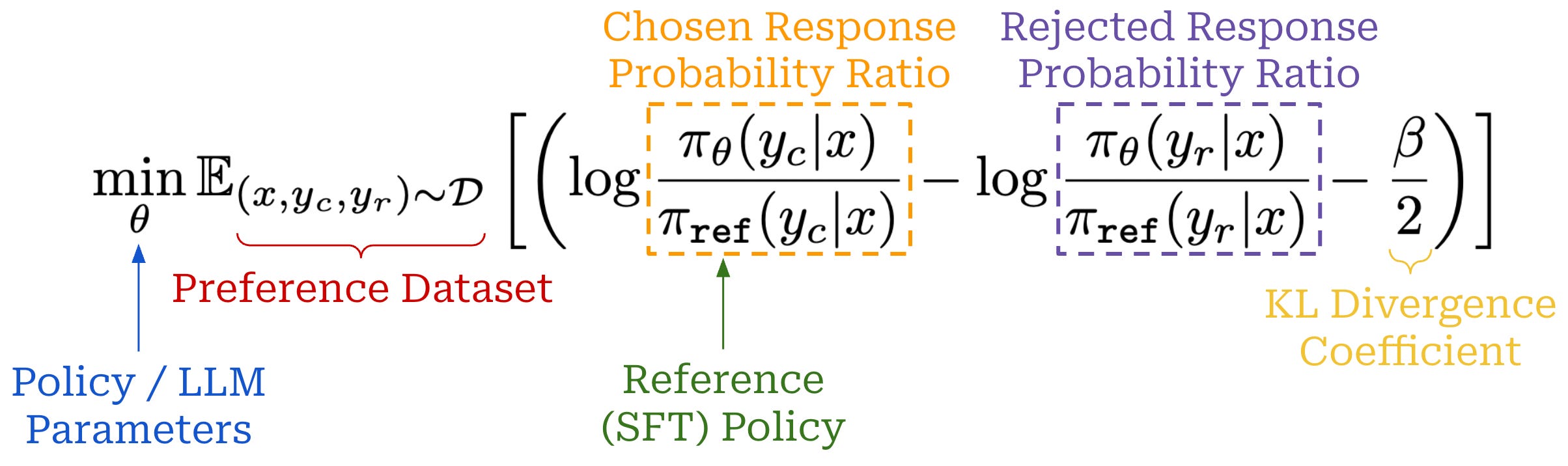
Experimental setup. All experiments in [5] evaluate models based on their win rate against a fixed policy and use the Identity Preference Optimization (IPO) algorithm, which uses the contrastive loss function shown above, for training. This algorithm is similar in nature to DPO. It can be used to align LLMs in an online or offline manner depending on how the training data is sampled.
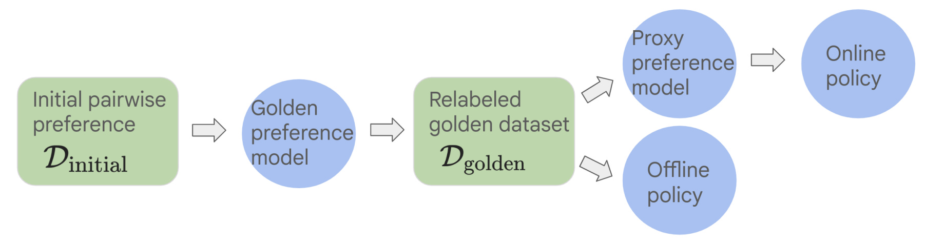
Specifically, we can use IPO in an online fashion by sampling on-policy data from the current policy during training, automatically scoring these completions with a reward model, and training the model over these online samples via the IPO training objective outlined above. A depiction of the differences between online and offline IPO is provided above. Online IPO is used as the online alignment technique in [5] instead of PPO-based RLHF for a few different reasons:
Implementing PPO is complex and expensive due to the requirement of an additional value function.
There is no clear way to formulate the PPO optimization process in an offline manner (though DPO was derived as an offline equivalent of PPO).
As discussed above, formulating IPO in either an online or offline fashion is relatively straightforward.
Given that PPO-based RLHF is the most widely-used online alignment algorithm, this choice to purely rely upon contrastive learning objectives is a clear deviation from mainstream alignment research. Additionally, analysis in [5] is performed over smaller (i.e., <1B parameter) models. Despite these issues, the learnings from this work still provide useful intuition that helps us to better understand the key distinctions between online and offline alignment algorithms.
Relative to offline algorithms, online alignment algorithms perform inference during training and require an additional training procedure for the reward model. For these reasons, we cannot compare online and offline algorithms based on their total compute budget—offline alignment in general will always be much cheaper. Instead, authors in [5] choose to compare policies in terms of their KL divergence from the SFT model, capturing how much the model changes during the alignment process (i.e., an optimization “budget”) in a compute-agnostic manner.
“Online algorithms tend to be more computationally intensive than offline algorithms, due to sampling and training an extra reward model… we do not prioritize compute as a main factor during comparison, and instead adopt the KL divergence between the RLHF policy and reference SFT policy as a measure of budget.”- from [8]
Comparing online and offline RL. To begin their analysis, authors present the results of online and offline alignment depicted in the figure below. Here, we see that there is a clear gap between the performance of models trained with online and offline alignment algorithms across all levels of possible KL divergence. These results are consistent across several different open alignment datasets8.
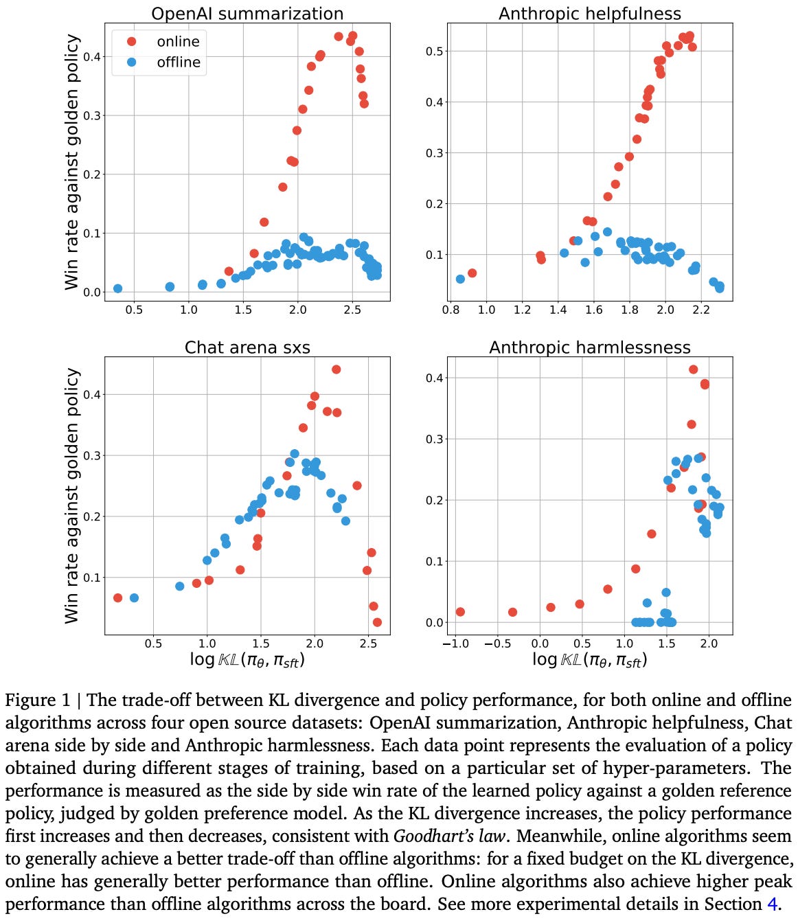
Based on the observed superiority of online alignment, authors in [5] propose the following potential explanations for the existence of this performance gap:
Data coverage: online algorithms outperform offline algorithms simply because they have more diverse data than the offline algorithm.
Sub-optimal data: offline algorithms perform worse because the completions in their dataset are generated by the SFT policy and are, therefore, of lower quality compared to on-policy samples generated during alignment9.
Better classification: offline algorithms train the policy to classify preferred completions in a preference pair, while online algorithms accomplish this via an explicit reward model. The performance gap may be due to the online algorithm’s explicit reward model performing this classification more accurately relative to the offline policy.
Contrastive loss: the contrastive objective used by offline algorithms like IPO and DPO—not their lack of on-policy sampling—may lead to the performance gap with online algorithms.
Scaling laws: the performance gap could potentially disappear as we scale up the size of the underlying policy.
Next, each of these hypotheses is studied in a series of ablation experiments that deeply analyze the difference between online and offline algorithms.
Data coverage. To study the impact of data coverage on alignment quality, we can collect all of the completions generated via on-policy sampling during online training to form a dataset for offline alignment. If we preserve the exact order in which this data was sampled, then online and offline alignment are identical—the models see the same data in the same order and, therefore, receive the same parameter updates. If we shuffle this data and use it for offline alignment, however, we see in [5] that this new data does not yield noticeably better results. As shown in the figure below, the offline algorithm performs similarly using an offline dataset and the shuffled dataset generated via on-policy sampling during online training.
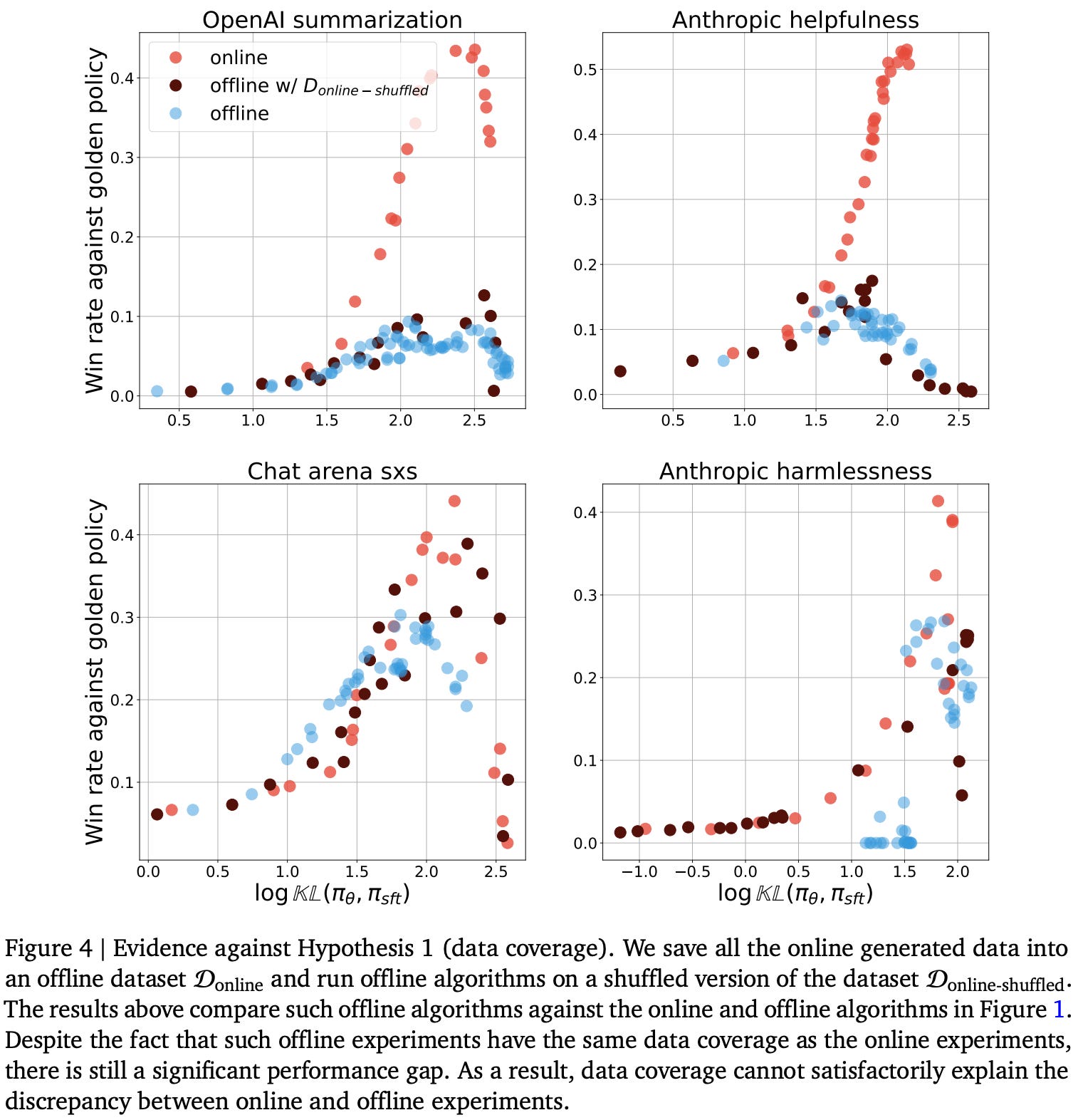
These results show that improving data coverage is not enough to overcome the performance limitations of offline alignment—data ordering is also important. However, this ordering need not be perfect. As we gradually increase the amount of shuffling in the on-policy samples, model performance remains stable up to a point, then rapidly deteriorates to the level observed with offline alignment.
“Offline algorithms, even when augmented with the same data coverage as the online algorithm, cannot obtain the same level of performance. This alludes to the importance of the exact sampling order obtained via on-policy sampling by a constantly evolving policy.” - from [5]
Sub-optimal data. We can easily test the impact of data quality on offline alignment algorithms by generating a preference dataset using a policy that is known to be high-quality. In [5], authors generate an offline training dataset using the final policy obtained via online alignment. When policies are trained over this dataset, there is only a slight improvement in quality; see below. Such a result indicates that the limitations of offline alignment algorithms are not purely due to the presence of lower-quality completions in their preference datasets.
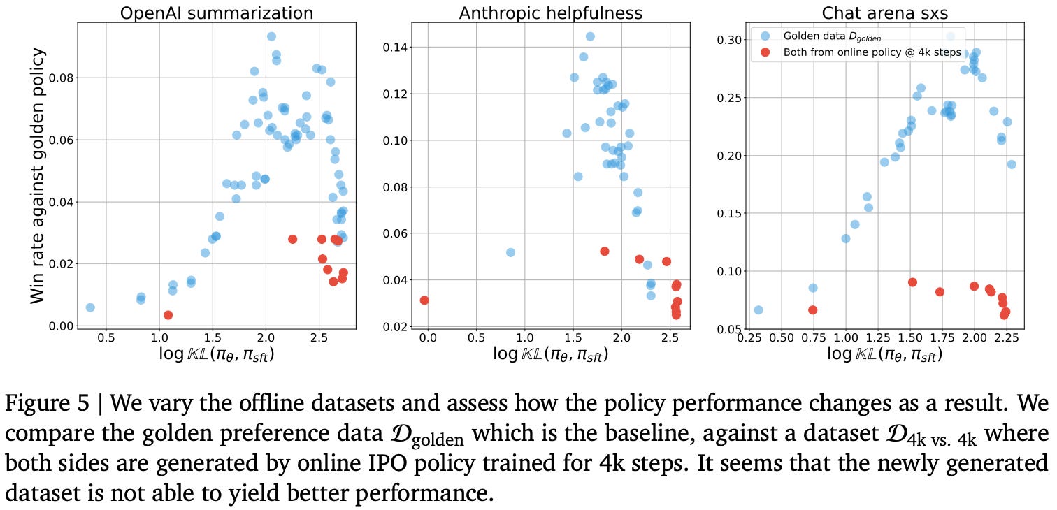
Classification accuracy. Authors in [5] demonstrate that explicit reward models used by online alignment algorithms achieve higher preference classification accuracy compared to the implicit reward estimate of an offline policy. However, little correlation is found between preference classification accuracy and model performance; in fact, the only observed correlation is slightly negative. Based on these findings, the authors conclude that the superior preference classification accuracy of online algorithms' explicit reward models is unlikely to be the primary factor behind the improved performance of online alignment methods.
Contrastive objective. To study whether the sub-par performance of offline alignment algorithms stems from their use of a contrastive loss function, authors derive a non-contrastive loss for offline alignment called Best-of-2. Put simply, the Best-of-2 training algorithm takes chosen completions for each preference pair in a dataset and runs SFT over these completions. When we train a model using the Best-of-2 loss over our standard offline preference dataset, there is no noticeable change in performance. However, adding online samples to Best-of-2 training—even when these samples are shuffled to remove the ordering from online alignment—nearly closes the performance gap with online techniques; see below.
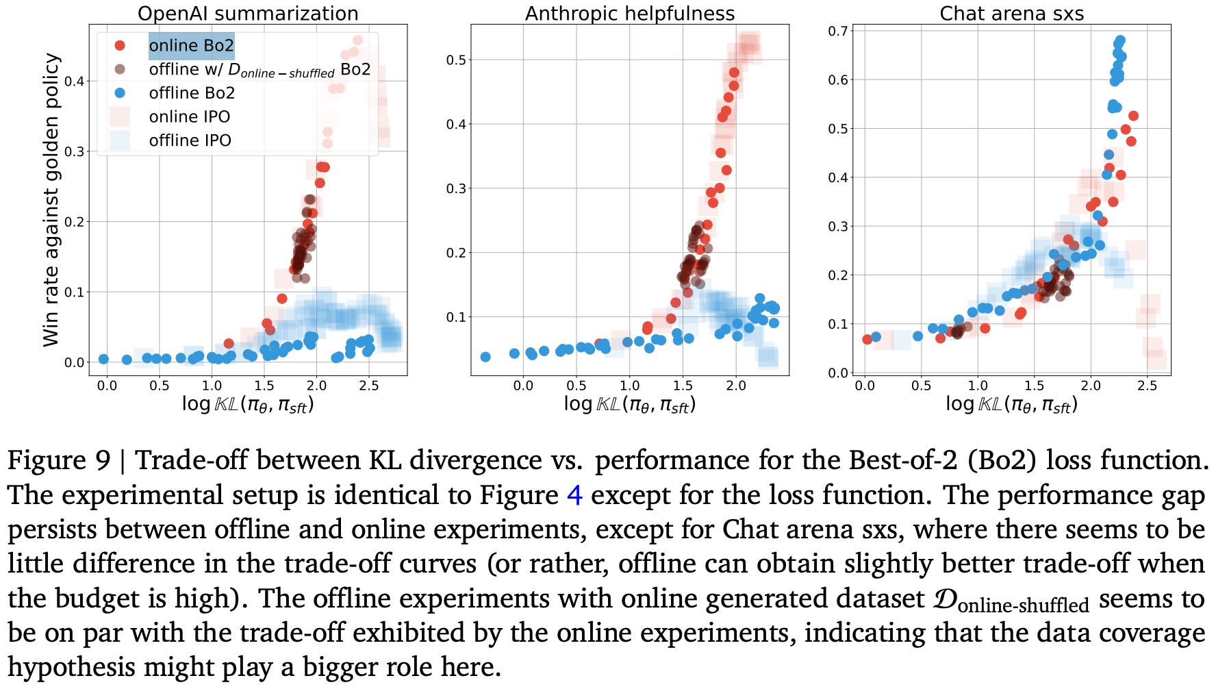
Such a result clearly demonstrates that data coverage is the key indicator of success for SFT, which motivates the inclusion of on-policy samples in SFT (i.e., rejection sampling). We can achieve impressive alignment results by simply including some level of on-policy data in offline training algorithms, forming practically effective LLM alignment baselines that are easy to implement.
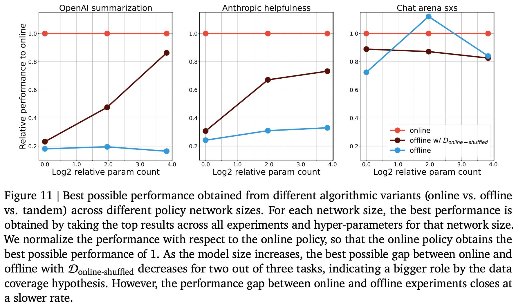
Does scaling up help? Authors end their analysis in [5] by studying the impact of model scale on the gap between online and offline alignment algorithms. In these experiments, we see that the gap between offline and online algorithms:
Decreases at larger scales.
Is more heavily related to data coverage at large scales.
More specifically, training larger models over a shuffled dataset of on-policy samples nearly closes the online-offline performance gap; see below. Such a finding did not hold in data coverage experiments with smaller models.
Key takeaway. The detailed alignment analysis in [5] leaves us with one key finding: on-policy sampling is important for high-quality alignment. There are many alternative explanations for the superiority of online alignment algorithms (e.g., data coverage or quality). However, these theories are debunked—at least at a smaller scale—by the many data ablations in [5], revealing that on-policy samples are the key contributor to the online-offline performance gap. This finding is very powerful, as it allows us to rethink the data sampling process used for offline alignment algorithms—we can improve the performance of offline techniques by incorporating (semi-)online data samples as described below!
“The dichotomy of online vs. offline is often inaccurate in practice, since an offline algorithm with a repeatedly updated data stream is effectively an online algorithm. As a result, offline learning can be made less likely to suffer from the shortcomings identified in this work, by being more careful with the data generation process in general.” - from [5]
Bridging Offline and Online Reinforcement Learning for LLMs [9]
“We study offline, semi-online, and online configurations, across both verifiable and non-verifiable tasks. By examining the transition from offline to online training (i.e., by altering the speed of periodic model syncing), we aim to understand how these methods can be optimized for improved performance and efficiency.” - from [9]
To granularly study the relationship between online and offline RL, authors in [9] finetune LLMs while smoothly transitioning the training process from an offline to an online setting. In other words, we bridge the gap between online and offline RL by testing training techniques that fall in the middle. By performing such tests over both verifiable (e.g., math) and non-verifiable domains (e.g., chat or instruction-following), we can gain an understanding of how on-policy sampling impacts the RL training process. More specifically, when we compare an on-policy GRPO setup to offline, semi-online, and on-policy variants of DPO, we learn that:
Online and semi-online techniques significantly outperform offline training.
Semi-online DPO nearly matches the performance of online DPO.
Put simply, we learn in [9] that online training is beneficial to model performance, but we can reap much of this benefit with a more efficient, semi-online approach.
Online, semi-online, and offline. For experiments in [9], authors train the Llama-3.1-8b-Instruct model using both on-policy GRPO and several variants of DPO. Specifically, we can create variants of DPO with varying degrees of on-policy sampling by defining a period s such that the policy being trained is used to generate fresh on-policy samples for DPO every s training iterations. In other words, we sync the parameters of the policy being trained and the policy used to sample completions for our preference data every s parameter updates; see below.
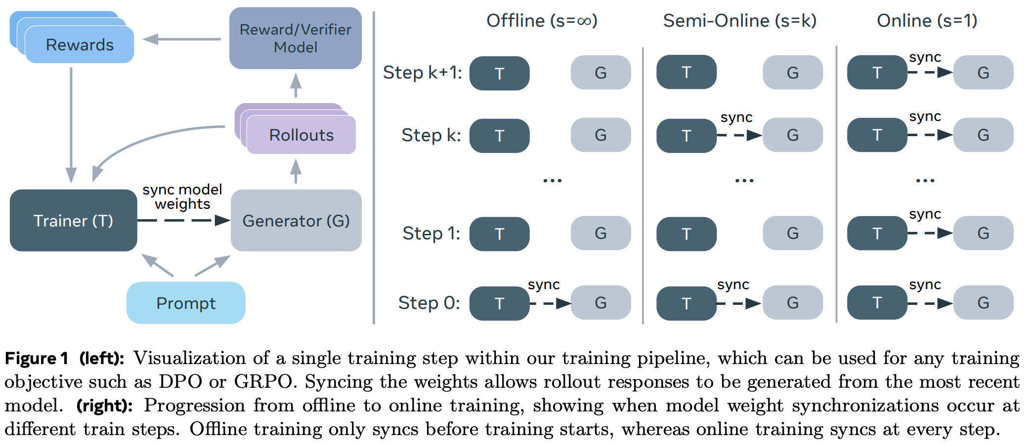
Notably, iterative forms of DPO—where we generate a new set of completions for training with the current model at each iteration—have been explored by prior work [10, 11]. However, these methods usually perform rough iterations, where new completions are sampled relatively infrequently. By varying the setting of s, we can explore arbitrary granularities of semi-online DPO, even including a fully on-policy DPO setting where s = 1. Put simply, we can bridge the gap between offline, semi-online, and online DPO by slowly decreasing s from ∞ to 1.
Experimental setup. Experiments are conducted in two possible domains:
A non-verifiable domain where training data is drawn from WildChat-1M10 and models are evaluated via LLM judges in terms of their chat capabilities (e.g., using AlpacaEval and Arena-Hard).
A math-focused, verifiable domain where training data is drawn from the NuminaMath dataset and evaluation is performed on several verifiable math benchmarks (e.g., Math500 and AMC23).
In the verifiable domain, the reward signal is obtained using the Math-Verify toolkit rather than exact string matching, which makes the reward more robust to variations in answer format11. The non-verifiable reward is derived from an off-the-shelf human preference reward model—Athene-RM-8b in particular—that is fixed throughout all experiments. To apply DPO in the verifiable domain, we simply generate several responses to each question, then choose a single correct and incorrect answer for each question to form preference pairs.
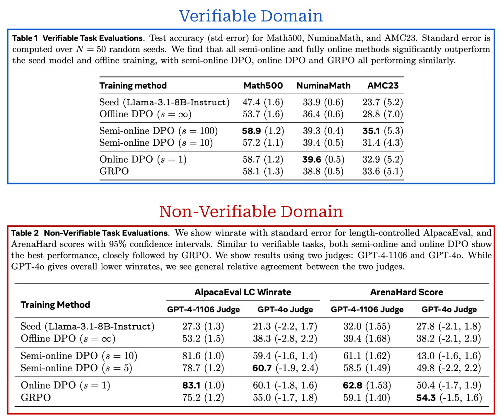
Is semi-online enough? The results of these experiments on both verifiable and non-verifiable tasks are shown above. Immediately, we see that training with an online or semi-online setup provides substantial gains over offline DPO in both domains. There is a clear performance gap between offline and online methods. But, the gap between online and semi-online settings is much less pronounced. In fact, online and semi-online DPO even outperform on-policy GRPO in some cases! These findings hold true even with relatively large values of s; e.g., in the verifiable domain s is increased to 100 with very promising results12.
“The efficiency gains of the semi-online variants opens up an interesting question of whether fully online RL is the only approach for post-training LLMs.” - from [9]
Such findings have interesting implications for the online-offline performance gap in RL. We see in [9] that there is a clear benefit to online sampling. However, we can potentially approximate this sampling more efficiently via a semi-online setup that intermittently collects fresh data instead of strict on-policy sampling.
Verifiable versus non-verifiable. Experiments are also performed in [9] to explore the interplay between verifiable and non-verifiable rewards, showing that the curriculum (or order) of rewards during RL training is important. If we compare settings in which the LLM is first trained on non-verifiable rewards then on verifiable rewards (NV → V) or vice versa (V → NV), we get better performance by first training on non-verifiable rewards (i.e., NV → V » V → NV).
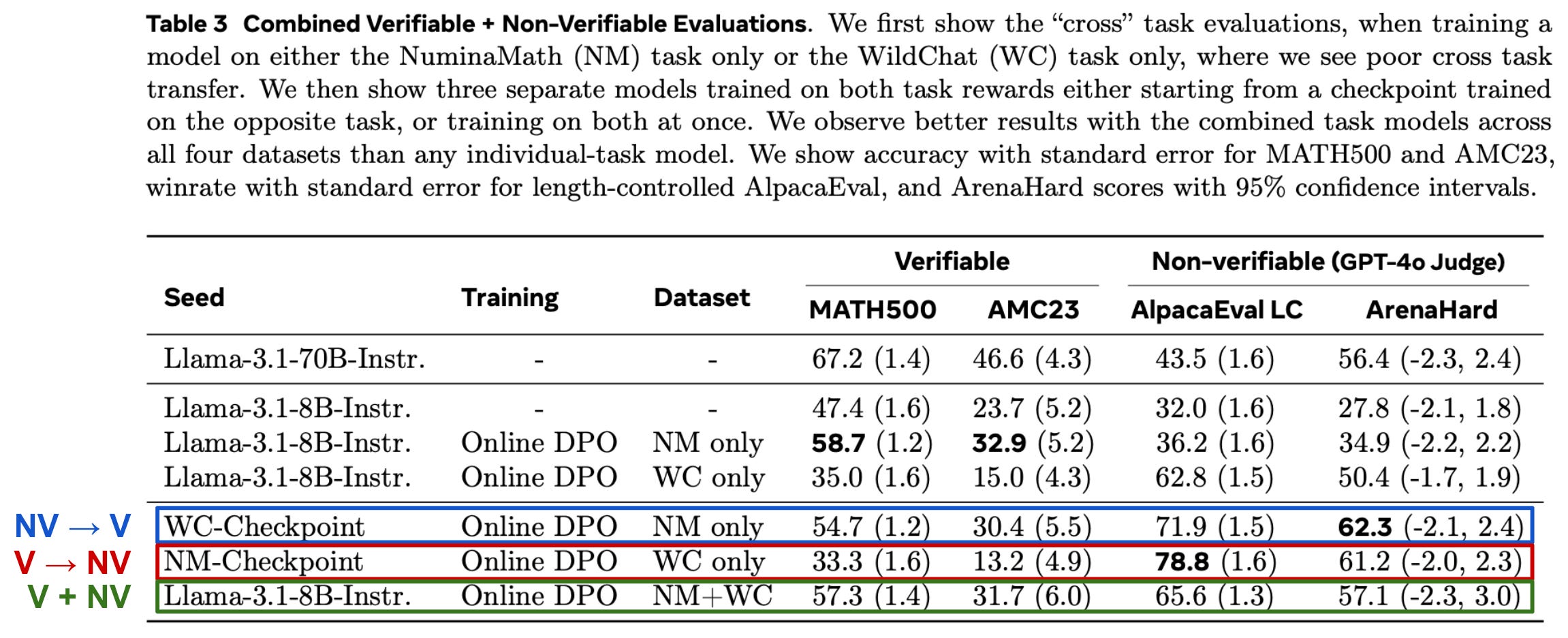
Training on non-verifiable rewards after the LLM has been trained on verifiable rewards leads to a noticeable performance deterioration in verifiable domains. In contrast, further training on verifiable rewards actually improves the performance of the LLM, even in non-verifiable domains; see above. If we combined both non-verifiable and verifiable rewards within a single training run (V + NV) the model also performs well, revealing that the simplest approach may be just mixing the disparate reward signals into a single, unified training run!
Conclusion
There are many alignment algorithms for LLMs, each varying in complexity and performance. Online algorithms have a clear performance benefit over offline alignment algorithms. In this overview, we have learned that this gap in performance primarily arises due to the use of on-policy sampling in online alignment algorithms, as well as other—arguably less significant—factors like negative gradients. Interestingly, however, we have also learned that much simpler and equally effective alignment algorithms can be derived by including on-policy samples in the training dataset used for offline alignment, forming semi-online algorithms that are practically effective and easy to implement.
New to the newsletter?
Hi! I’m Cameron R. Wolfe, Deep Learning Ph.D. and Senior Research Scientist at Netflix. This is the Deep (Learning) Focus newsletter, where I help readers better understand important topics in AI research. The newsletter will always be free and open to read. If you like the newsletter, please subscribe, consider a paid subscription, share it, or follow me on X and LinkedIn!
Bibliography
[1] Rafailov, Rafael, et al. "Direct preference optimization: Your language model is secretly a reward model." Advances in neural information processing systems 36 (2023): 53728-53741.
[2] Ivison, Hamish, et al. "Unpacking dpo and ppo: Disentangling best practices for learning from preference feedback." Advances in neural information processing systems 37 (2024): 36602-36633.
[3] Ivison, Hamish, et al. "Camels in a changing climate: Enhancing lm adaptation with tulu 2." arXiv preprint arXiv:2311.10702 (2023).
[4] Tunstall, Lewis, et al. "Zephyr: Direct distillation of lm alignment." arXiv preprint arXiv:2310.16944 (2023).
[5] Tang, Yunhao, et al. "Understanding the performance gap between online and offline alignment algorithms." arXiv preprint arXiv:2405.08448 (2024).
[6] Xu, Shusheng, et al. "Is dpo superior to ppo for llm alignment? a comprehensive study." arXiv preprint arXiv:2404.10719 (2024).
[7] Tajwar, Fahim, et al. "Preference fine-tuning of llms should leverage suboptimal, on-policy data." arXiv preprint arXiv:2404.14367 (2024).
[8] Azar, Mohammad Gheshlaghi, et al. "A general theoretical paradigm to understand learning from human preferences." International Conference on Artificial Intelligence and Statistics. PMLR, 2024.
[9] Lanchantin, Jack, et al. "Bridging Offline and Online Reinforcement Learning for LLMs." arXiv preprint arXiv:2506.21495 (2025).
[10] Yuan, Weizhe, et al. "Self-rewarding language models." arXiv preprint arXiv:2401.10020 3 (2024).
[11] Pang, Richard Yuanzhe, et al. "Iterative reasoning preference optimization." Advances in Neural Information Processing Systems 37 (2024): 116617-116637.
[12] Shao, Zhihong, et al. "Deepseekmath: Pushing the limits of mathematical reasoning in open language models." arXiv preprint arXiv:2402.03300 (2024).
[13] Mukobi, Gabriel, et al. "Superhf: Supervised iterative learning from human feedback." arXiv preprint arXiv:2310.16763 (2023).
[14] Gulcehre, Caglar, et al. "Reinforced self-training (rest) for language modeling." arXiv preprint arXiv:2308.08998 (2023).
[15] Hu, Jian, et al. "Aligning language models with offline learning from human feedback." arXiv preprint arXiv:2308.12050 (2023).
[16] Lambert, Nathan, et al. "Tulu 3: Pushing frontiers in open language model post-training." arXiv preprint arXiv:2411.15124 (2024).
[17] Ouyang, Long, et al. "Training language models to follow instructions with human feedback." Advances in neural information processing systems 35 (2022): 27730-27744.
[18] Rafailov, Rafael, et al. "Direct preference optimization: Your language model is secretly a reward model." Advances in neural information processing systems 36 (2023): 53728-53741.
[19] Ethayarajh, Kawin, et al. "Kto: Model alignment as prospect theoretic optimization." arXiv preprint arXiv:2402.01306 (2024).
[20] Xu, Haoran, et al. "Contrastive preference optimization: Pushing the boundaries of llm performance in machine translation." arXiv preprint arXiv:2401.08417 (2024).
[21] Huang, Shengyi, et al. "The n+ implementation details of rlhf with ppo: A case study on tl; dr summarization." arXiv preprint arXiv:2403.17031 (2024).
This can be accomplished using a completion-only loss collator.
There are a few different ways this selection can be performed. For example, we can select the top completion for each prompt, or we can select the top-scoring completions across all prompts; see here for details.
In other words, the output is a vector of size eight to which a softmax function has been applied to form a probability distribution over these eight possible outcomes.
GRPO is not listed in this table due to the fact that both [7] and the GRPO paper [12] were published at very similar times.
The LLM before alignment already generates completions that are near the average length. In contrast, the LLM does not generate minimum (or zero) length completions, so learning to generate such responses requires probability mass to be moved into a new region that was previously unlikely.
This sensitivity is due to the fact that maximum likelihood algorithms do not have any explicit mechanism to protect against off-policy sampling, whereas PPO has the clipping operation and KL divergence that help to maintain the trust region.
As an example of how we can obtain preference data via web scraping, the Stack Exchange Preferences dataset takes questions from Stack Overflow with at least two answers and ranks answers based on implicit feedback (e.g., likes or upvotes).
Specifically, this work uses the OpenAI summarization, Anthropic Helpful and Harmless (hh-rlhf), and the Chatbot arena preference dataset.
We should note that one can make a similar argument against online algorithms! The reward model used in online algorithms is also trained over a fixed dataset, which can lead to similar limitations in the performance of online algorithms.
This is a general chat and instruction-following benchmark that is comprised of ~1M user interactions with ChatGPT.
For example, an LLM could provide an answer of 0.5 or 1/2 to a math question. Both of these answers would be correct, but one of them would likely be marked as wrong if we are verifying our reward via exact string match. For this reason, using a more robust validation system for mathematical expressions is helpful.
The value of s is much larger in the verifiable domain compared to the non-verifiable domain. Authors in [9] make this choice because the non-verifiable dataset is small and a setting of s = 32 spans a full epoch over the data. Therefore, the training process is not stable with larger values of s in the non-verifiable domain.
again, super dense and great article, thx!
I wonder if these algorithms use network analysis like Eigen vector and degree centrality