
Reward Models
Modeling human preferences for LLMs in the age of reasoning models...


Reward models (RMs) are a cornerstone of large language model (LLM) research, enabling significant advancements by incorporating human preferences into the training process. Despite their critical role, RMs are often overlooked. Practical guidance on how to train and use them effectively remains scarce—particularly as RM-free techniques like reinforcement learning with verifiable rewards gain popularity. Nevertheless, training LLMs with PPO-based reinforcement learning continues to be a crucial factor in developing top foundation models. In this overview, we will build a deep understanding of RMs from the ground up, clarifying their historical and ongoing significance in the rapidly evolving LLM ecosystem.
What is a Reward Model?
“Reward models broadly have been used extensively in reinforcement learning research as a proxy for environment rewards… The most common reward model predicts the probability that a piece of text was close to a preferred piece of text from the training comparisons.” - RLHF book
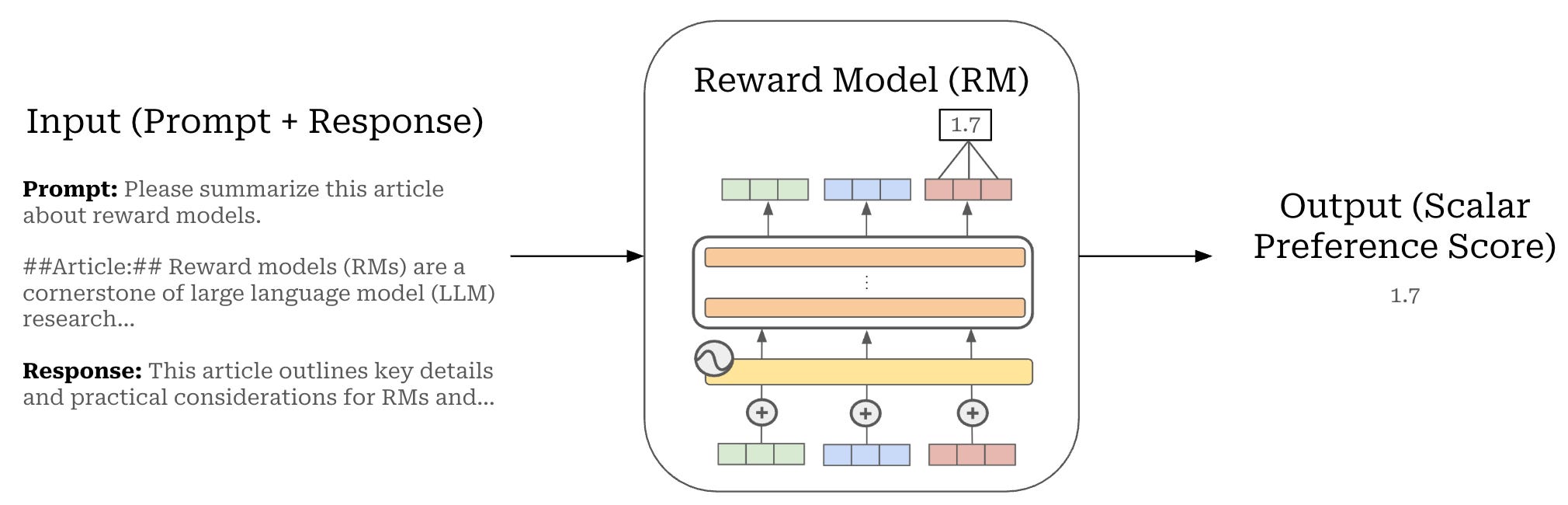
Reward models (RMs) are specialized LLMs—usually derived from an LLM that we are currently training—that are trained to predict a human preference score given a prompt and a candidate completion as input; see above. A higher score from the RM indicates that a given completion is likely to be preferred by humans.
As a first step, we must build a fundamental understanding of reward models (RMs), how they are created, and how we use them in the context of LLMs. In this section, we will focus on understanding the following:
The motivation for RMs, as derived from statistical models of preferences.
The architecture and structure used by most RMs.
The training process for an RM.
To understand how RMs are used, we need more context around reinforcement learning (RL) and LLM post-training, which will be covered in the next section.
The Bradley-Terry Model of Preference
The standard implementation of an RM is derived from the Bradley-Terry model of preference—a statistical model used to rank paired comparison data based on the relative strength or performance of items in the pair. Given two events i and j drawn from the same distribution, the Bradley-Terry model defines the probability that item i wins—or is preferred—compared to item j as follows:

In the context of LLMs, items i and j are two completions generated by the same LLM and from the same prompt (i.e., these completions are sampled from the same distribution). The RM assigns a score to each of these completions, then we use the above expression from the Bradley-Terry model to derive a probability that completion i is preferred to completion j. Put simply, we use the Bradley-Terry model to express probabilities for pairwise comparisons between two completions.
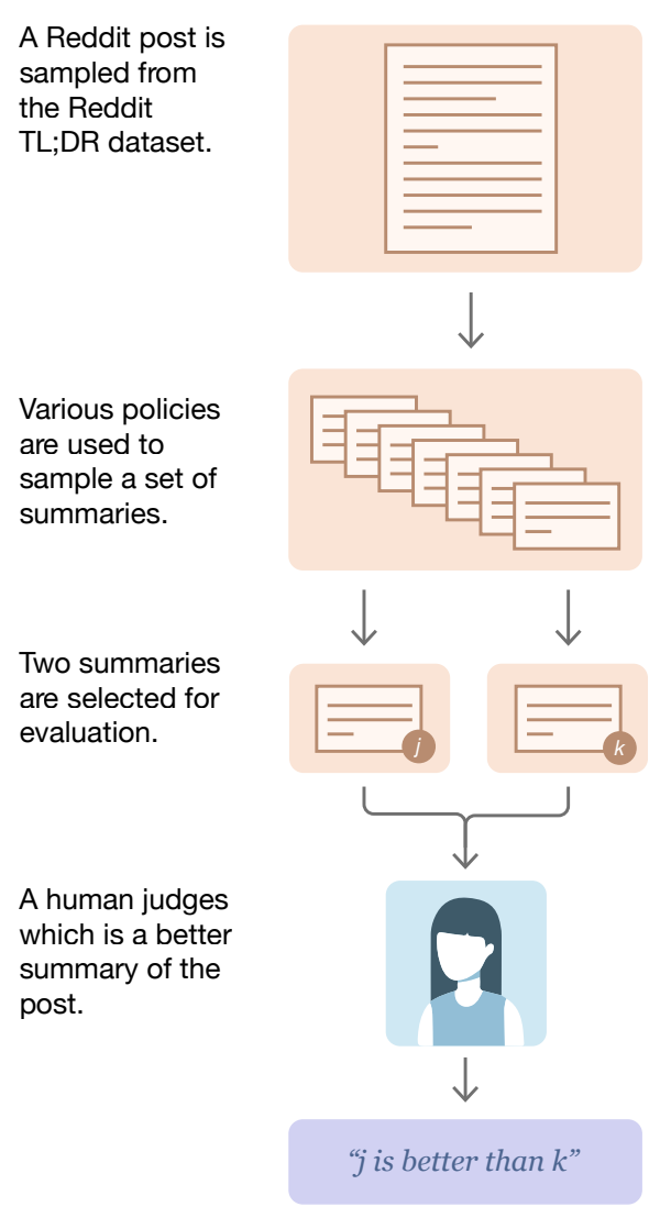
Preference data. Pairwise preference data is used—and has been used for quite some time [14]—extensively in LLM post-training. Such data is comprised of many different prompts, and we aim to maximize the diversity of prompts in our data. The prompt distribution should be representative of prompts a model will see in the wild. For each prompt, we have a pair of candidate completions1, where one completion has been identified—usually by a human, but sometimes by a model—as preferable to the other; see above. A dataset of prompts with associated chosen and rejected completions is referred to as a (human) preference dataset.
How do RMs work?
We know that RMs are based upon the Bradley-Terry model of preference, but there are many ways that we could implement such a statistical model practically. In the domain of LLMs, these models are implemented—perhaps unsurprisingly—with an LLM. Compared to standard (generative) decoder-only LLMs, however, RMs modify both the underlying architecture and training objective.

RM architecture. An RM takes a prompt-completion pair from an LLM as input and outputs a (scalar) preference score. In practice, the RM is implemented with an LLM by adding a linear head to the end of the decoder-only architecture; see above. Specifically, the LLM outputs a list of token vectors—one for each input token vector—and we pass the final vector from this list through the linear head to produce a single, scalar score. We can think of the RM as an LLM with an extra classification head used to classify a given completion as preferred or not preferred.
Training process. The parameters of the RM are usually initialized with an existing policy2, which we will refer to as the RM’s “base” model. Several choices exist for the policy with which to initialize the RM; e.g., the LLM being trained or a prior version of this model like the pretrained base or SFT model. Once the RM is initialized, we add the linear head to this model and train it over a preference dataset (i.e., pairs of chosen and rejected model responses to a prompt).
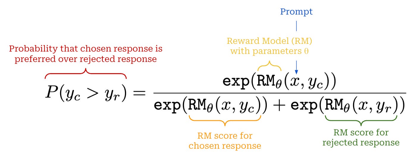
Given a preference pair, we want our RM to assign a higher score to the chosen response relative to the rejected response. In other words, the optimal RM should maximize the probability that the chosen response is preferred to the rejected response. As we learned before, we can use the Bradley-Terry model to express this probability; see above. Rearranging this probability expression, we can derive the loss function shown below, which is a pairwise ranking loss that simply encourages the model to assign a higher score to the chosen response.
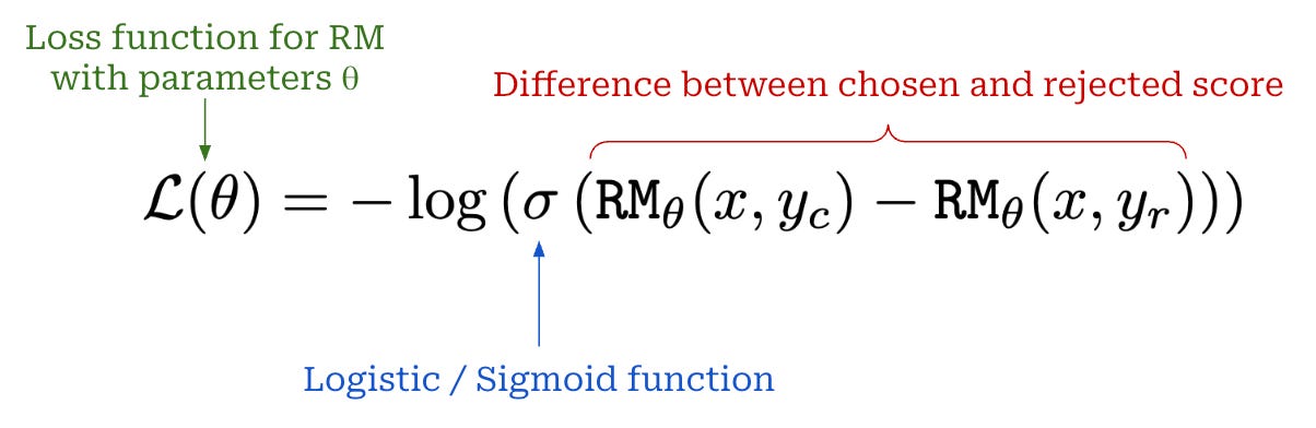
We can think of this as a negative log likelihood (NLL) loss, where the probability for NLL is given by the Bradley-Terry model. A visualization of the landscape for this loss is shown below, where we see that the loss is minimized when the chosen score is maximized and the rejected score is minimized. By empirically minimizing this loss function over a large preference dataset, we can (approximately) maximize the expected probability that chosen responses are preferred to rejected responses.

Normalizing the reward. After training, the RM outputs unnormalized scalar values. To lower the variance of the reward function (i.e., make sure the RM’s output falls in a standard range), we can normalize the RM’s output such that it assigns an average reward of zero over our preference dataset used for training. Authors in [14] mention using this reward normalization approach.
“At the end of training, we normalize the reward model outputs such that the reference summaries from our dataset achieve a mean score of 0.” - from [14]
Implementing an RM
To make this discussion more practical, let’s learn how RMs—including both the architecture and loss function—can be implemented using common deep learning frameworks. An RM is just a classification model— it performs text classification over a sequence of text. Given a prompt and response as input, the RM predicts the likelihood (i.e., a single scalar score) that this prompt-response pair is preferred.
Toy example. We can implement this via an abstraction like HuggingFace’s AutoModelForSequenceClassification. An implementation of a small (BERT-based) RM that can be run locally is provided below, where we:
Create the RM using
AutoModelForSequenceClassification.Compute the RM’s output—in the form of a single logit—for all chosen and rejected sequences3.
Compute the RM’s loss as described above.
from transformers import (
    AutoTokenizer,
    AutoModelForSequenceClassification,
)
import torch

# Load a tiny model for sequence classification
model_name = "google-bert/bert-base-uncased"
tokenizer = AutoTokenizer.from_pretrained(
    model_name,
    trust_remote_code=True,
)
model = AutoModelForSequenceClassification.from_pretrained(
    model_name,
    trust_remote_code=True,
)

# Chosen prompt-response sequences
chosen_seqs = [
    "I love deep (learning) focus!",
    "Cameron is great at explaining stuff",
    "AGI is coming very soon...",
]

# Rejected prompt-response sequences
rejected_seqs = [
    "I'm not a fan of deep (learning) focus",
    "Cameron doesn't know what he's talking about",
    "AGI is fake and LLMs can't reason!",
]

# Tokenize the chosen / rejected sequences
chosen_inps = tokenizer(
    chosen_seqs,
    return_tensors="pt",
    padding=True,
)
rejected_inps = tokenizer(
    rejected_seqs,
    return_tensors="pt",
    padding=True,
)

# Compute the RM's output
rewards_chosen = model(**chosen_inps).logits[:, 0]
rewards_rejected = model(**rejected_inps).logits[:, 0]

# Compute the RM's loss
loss = -torch.nn.functional.logsigmoid(
    rewards_chosen - rewards_rejected
).mean()
print(loss)
From here, we train the RM similarly to any other model; i.e., by i) looping over a preference dataset, ii) computing the loss as outlined above, iii) obtaining a gradient via backpropagation, iv) performing a gradient update and v) repeating.
Real RM training example. For a more practical view of what training an RM looks like at an LLM research lab, we can look at the RM training script in AI2’s OpenInstruct. This script implements distributed training of an RM—based upon OLMo-2 or OLMoE—using accelerate. The script is quite simple, and most of the code is actually just configuring the training process. We can parse through this training script to find the core RM training loop, copied below for reference.
for _ in range(args.num_train_epochs):
    for data in dataloader:
        training_step += 1

        # Concat the chosen / rejected sequences
        query_responses = torch.cat(
            (
                data[CHOSEN_INPUT_IDS_KEY],
                data[REJECTED_INPUT_IDS_KEY]
            ),
            dim=0,
        )
        with accelerator.accumulate(model):
            # Predict reward for each sequence with RM
            _, predicted_reward, _ = get_reward(
                model,
                query_responses,
                tokenizer.pad_token_id,
                0,
            )

            # Parse chosen / rejected rewards from output
            chosen_reward = predicted_reward[
                :data[CHOSEN_INPUT_IDS_KEY].shape[0]
            ]
            rejected_reward = predicted_reward[
                data[CHOSEN_INPUT_IDS_KEY].shape[0] :
            ]

            # Compute loss and gradient for RM
            loss = -F.logsigmoid(chosen_reward - rejected_reward).mean()
            accelerator.backward(loss)

            # Perform parameter update for RM
            optimizer.step()
            optimizer.zero_grad()
As we can see, this code, which is used for training large-scale RMs at a top research lab, is not much different from our toy example! Of course, the training loop is largely made simple by abstractions provided by modern deep learning packages like HuggingFace. However, the key takeaway here is that the concepts we have learned so far directly translate to practical training and usage of RMs.
Different Types of RMs
So far, we have focused on the standard form of an RM, typically referred to as a classifier-based RM. However, RMs are just models that predict a preference score given a prompt and response, which we can implement in many ways. For example, we can train a custom classifier like ArmoRM to serve as an RM.

LLM-as-a-Judge models can also be used as an RM by simply prompting an LLM judge to provide a preference score; see above. These preference scores can then be taken as the reward signal during training with RL. For a more in-depth overview of LLM-as-a-Judge, please see the article linked below.

Alternatively, we can use LLM judges to collect synthetic preference data—using prompts like the one shown below from AlpacaEval—and train an RM normally over this synthetic data, as is done by Constitutional AI [10] and RLAIF [11].

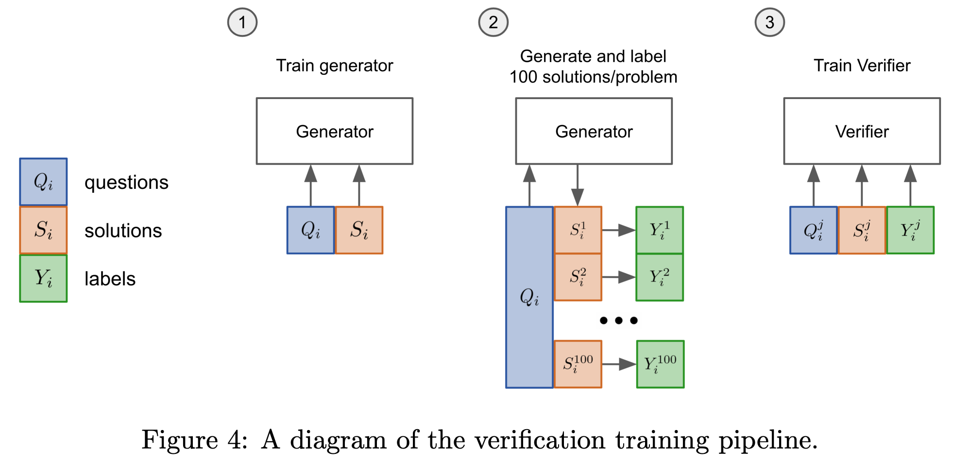
Outcome Reward Models (ORMs) [12] and Process Reward Models (PRMs) [11] are two other commonly-used variants of RMs in the literature. ORMs, which are mostly used for reasoning tasks, predict the probability that a completion is the correct answer to a task. To train an ORM, we collect a preference dataset similarly to before, but each preference pair contains both an incorrect and a correct answer to a given question. Unlike a standard RM that predicts the reward at a sequence level, the ORM predicts correctness on a per-token basis.
“Our verifiers are language models, with a small scalar head that outputs predictions on a per-token basis.” - from [12]
Like ORMs, PRMs are used primarily for reasoning tasks and predict more granular outputs, but PRMs make predictions after every step of the reasoning process rather than after every token. Although PRMs have been used in a variety of papers, collecting training data for PRMs is difficult, as they require granular supervision (i.e., a correctness signal at each step of the reasoning process).
“PRMs are reward models trained to output scores at every step in a chain of thought reasoning process. These differ from a standard RM that outputs a score only at an EOS token or a ORM that outputs a score at every token. Process Reward Models require supervision at the end of each reasoning step.” - source
The Role of Reward Models in Post-Training

Early post-ChatGPT LLMs were almost always post-trained using the three-step alignment procedure (shown above) proposed by InstructGPT [3]. This procedure is comprised of the following three steps:
Supervised finetuning (SFT)—a.k.a. instruction finetuning (IFT)—trains the model using next-token prediction over examples of good completions.
A reward model (RM) is trained over a human preference dataset.
Reinforcement learning (RL) is used to finetune the LLM by using the output of the RM as a training signal.
Collectively, steps two and three in this procedure are called reinforcement learning from human feedback (RLHF)—we use a reinforcement learning (RL) optimizer to finetune the LLM and incorporate human feedback via preference labels.
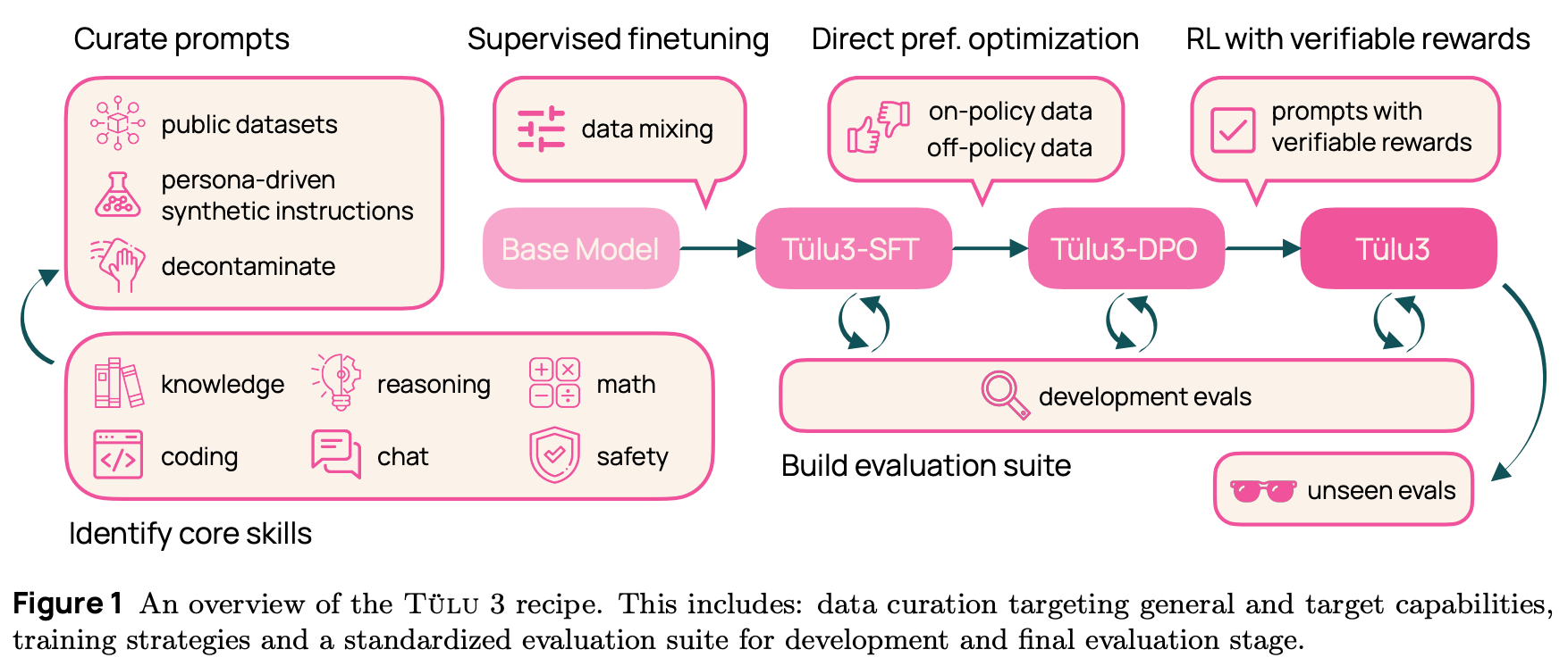
Today, the story is a bit more complicated; an example of a more modern post-training pipeline (used for Tulu-3 [4]) is provided above. Key differences from the original three step alignment procedure include:
The SFT phase—although still very common— is not always used, especially for recent reasoning models; e.g., some variants of DeepSeek-R1 forgo SFT and apply RL directly to the pretrained model.
RL training is usually performed in several rounds, where fresh data is collected for each round to further improve the LLM’s capabilities.
Several variants of RL (and non-RL-based alternatives) are used—potentially in tandem—that may or may not require an RM.
Despite the extra complexity, data quality remains the key determinant of successful post-training even today. In this section, we will cover RL training frameworks at a high level, focusing on the role (if any) of RMs in each of them.
RL Training Strategies for LLMs
For those who are unfamiliar with the high-level setup used for training LLMs with RL, please see the overview below. A basic understanding of RL in the context of LLMs is a necessary prerequisite for this discussion.

RL for LLMs. There are two broad categories of reinforcement learning (RL) training that are heavily leveraged by LLMs: RLHF (i.e., steps two and three of the post-training setup that we outlined above) and reinforcement learning with verifiable rewards (RLVR). These two variants of RL are depicted below.

From an RL perspective, these techniques are similar. They follow the same high-level training setup and both use RL optimizers based upon policy gradient algorithms4 to derive parameter updates. The primary difference between these techniques lies in how we define the reward:
In RLHF, the reward comes from the RM, which provides a human preference score for each of the completions provided by the LLM.
RLVR uses deterministic (or verifiable) rewards, where the answer provided by the LLM is marked as either correct or incorrect.
Notably, the deterministic—usually rules-based—rewards in RLVR eliminate the need for an RM! Usually, rewards are derived by extracting the LLM’s final answer from its generated output and comparing this answer (e.g., via exact string match or some form of fuzzy matching) to a known, ground truth answer. From this comparison, we can determine whether the LLM’s output is correct or not and use this binary signal as a reward for training with RL.
RLHF vs RLVR. In more recent frontier models, both styles of RL play a role in the post-training process. We still perform the three step post-training procedure (SFT → RLHF), which teaches the LLM correct formatting and aligns it to human preferences. However, we now have an additional RLVR step that boosts reasoning capabilities and performance on verifiable tasks; see below.

More generally, the amount of compute being invested into RL finetuning—and RLVR in particular—is also rapidly increasing. This change is motivated by recent results on reasoning models that show clear scaling laws of model performance with respect to the amount of compute used for RL training; see below.

“RLHF is a complex and often unstable procedure… we introduce a new parameterization of the reward model in RLHF that [allows] us to solve the standard RLHF problem with only a simple classification loss.” - from [6]
Direct alignment. RLVR is not the only way to avoid using an RM. In fact, we can still align a model to human preferences—similarly to RLHF—while foregoing the RM completely. Such techniques are referred to as direct alignment algorithms, and the most widely-used algorithm in this class is direct preference optimization (DPO) [6]. Not only do direct alignment algorithms like DPO forego the RM while optimizing the same training objective as RLHF, but they avoid RL training altogether. A comparison between RLHF and DPO is provided below.
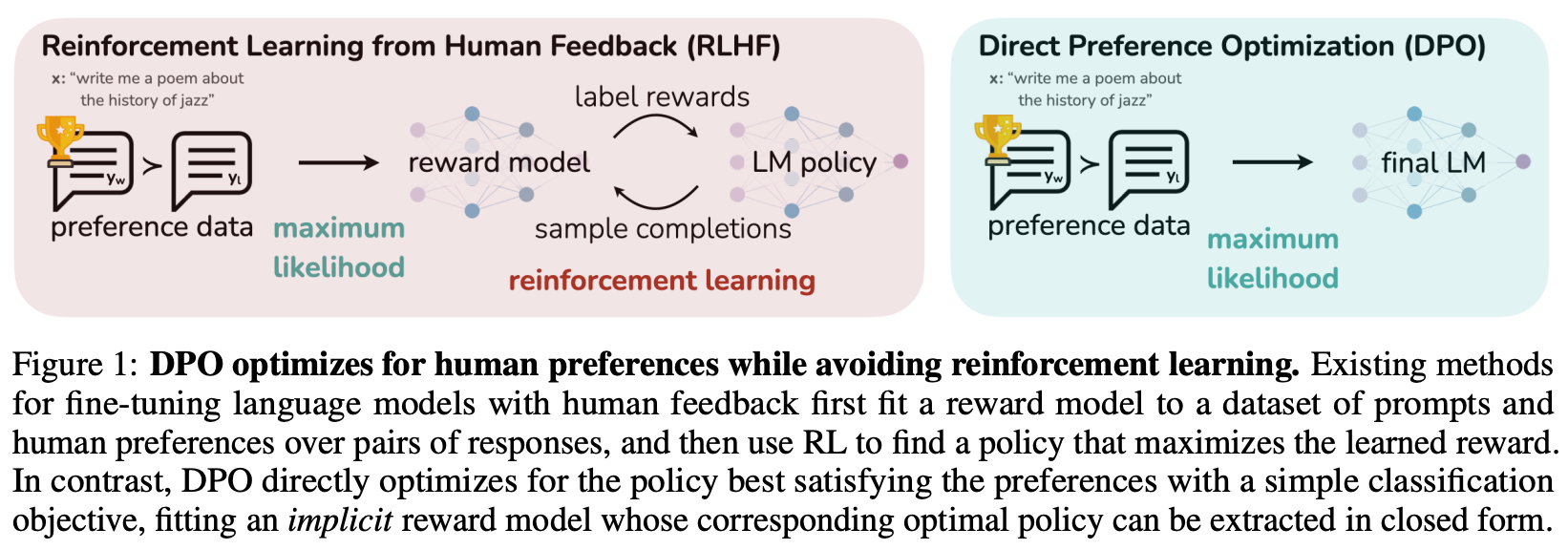
The loss function used for training in DPO is presented below. As we can see, this loss function looks very similar to the loss function used by an RM. However, we are no longer predicting the reward with an RM. Instead, we directly use our policy to estimate a reward implicitly by using the probabilities of chosen and rejected completions assigned by the current policy and a reference policy. Intuitively, this loss is minimized when the log-ratio of the chosen completion is larger than that of the rejected completion. DPO trains the current policy to assign higher (implicit) rewards to chosen responses relative to rejected responses.

DPO does not require the creation of an intermediate RM. However, the loss function is still derived from the Bradley-Terry model, and we are still learning an RM. The key distinction here is that the RM is learned implicitly rather than explicitly; hence the title of the DPO paper [6] “Your Language Model is Secretly a Reward Model”. We can directly obtain this implicit reward estimate from a DPO model similarly to an RM. For a full derivation and analysis of DPO; see here.
Why are RMs useful?
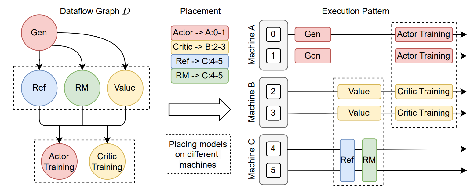
Without a doubt, using an RM adds extra complexity to the LLM training process. First, we need to train a separate model over a large preference dataset, which already introduces added costs and complexity. From here, this model is used in an online fashion during RL training—the RM scores completions generated by the current policy during training. Given that the RM is also an LLM, this means that we have to separately host and run inference for a separate LLM during training, which can be difficult to efficiently orchestrate; see above.
“We find that the neural RMs may suffer from reward hacking in the large-scale reinforcement learning process. Retraining the reward model needs additional training resources and it complicates the whole training pipeline.” - from [7]
Reward hacking. Going further, RMs are subject to reward hacking. The RM may spuriously assign high rewards to low quality completions or—more generally—be exploited in a way that allows the policy to receive high rewards without actually solving the desired task. Interestingly, reward hacking is a key limitation that prevents scaling up training with RLHF—our policy will eventually find an exploit for the RM if we continue to train it for long enough. In contrast, verifiable rewards are more difficult (though not impossible) to hack, allowing reasoning models to be trained more extensively (i.e., for more iterations) when using RLVR.
Should we avoid RMs? Given the added costs and complexity of RMs, we might wonder: Should we just avoid RMs altogether? There is no definitive answer to this question. Impressive results have been achieved via RLVR, and we can still align models to human preferences with techniques like DPO that avoid an RM. Many works have argued whether there is (or is not) a performance gap between RLHF and DPO with differing results. Whether DPO is an effective RM-free preference tuning alternative is dependent on the use case, but the fact that there is a gap in performance between these techniques is generally accepted to be true.
“The prevalence of RLHF stems from its efficacy at circumventing one of the greatest difficulties in integrating human values and preferences into language models: specifying an explicit reward” - from [1]
The utility of RMs. Despite these findings, we should not lose sight of the fact that RMs are an incredibly important and powerful concept. One of the most difficult tasks in any form of RL training is specifying a reward. For LLMs, this task is especially difficult—how do we explicitly define what constitutes a “good” response from an LLM? Unfortunately, there is no single property or quality that can be used. The scope of valid model responses is nearly infinite.
With RMs, we circumvent the problem of specifying an explicit reward by distilling this process into a simpler task of asking humans to provide preference feedback (i.e., choosing among pairs of model responses); see below.
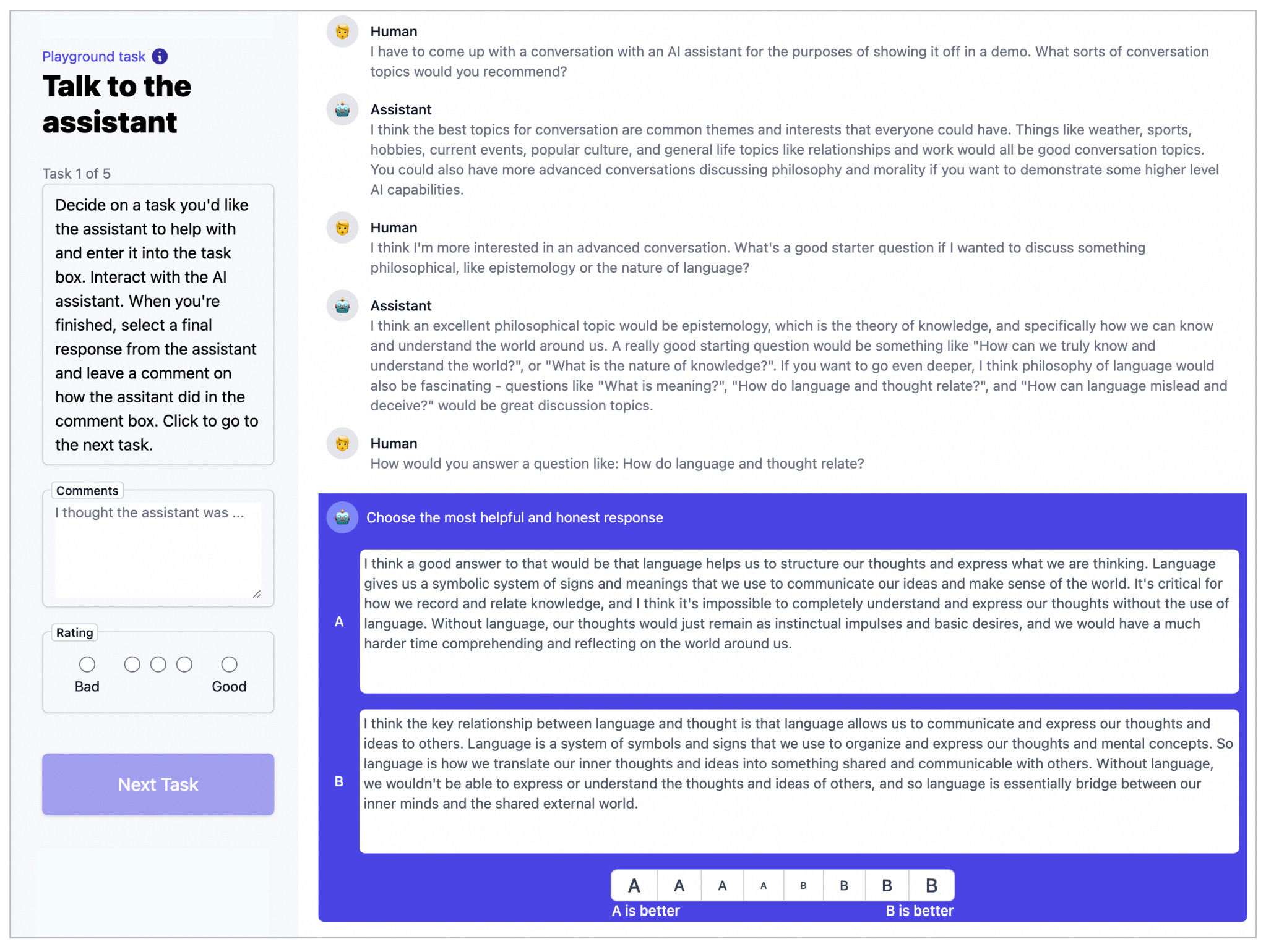
Choosing the better model in a pair is a much simpler task compared to manually writing or evaluating individual model responses—the human just has to provide a binary preference. We can train an RM over this preference feedback, allowing us to derive a reward for RL training without ever making an explicit specification of the reward. Such an approach provides us with a flexible and effective approach for training LLMs with generic human feedback, which is transformational.
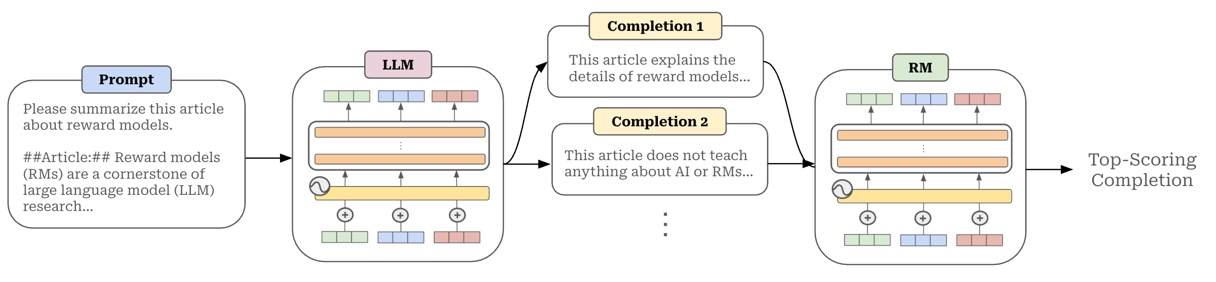
Other use cases for RMs. Beyond their use in RL training, RMs have a variety of other use cases. For example, RMs are commonly used for i) Best-of-N sampling and inference-time scaling (see above), ii) evaluation, iii) rejection sampling, iv) data filtering and much more! Despite these many use cases, we usually evaluate the performance of an RM based upon:
Accuracy: an RM’s ability to correctly identify the chosen response in a pair.
Downstream performance: the performance of an LLM that is RL finetuned with a particular RM.
Inference-time scaling: the performance boost achieved by using a particular RM in a Best-of-N sampling pipeline.
Reward Models in Practice
Now that we have an understanding of RMs, we will study some recent papers on this topic. Specifically, we will focus on RewardBench [1], which is a benchmark for evaluating the effectiveness of RMs. This benchmark has been used to evaluate hundreds of different RMs across a variety of use cases, allowing us to derive useful takeaways for effectively training and using RMs in practice. Recently, a new version of RewardBench—called RewardBench 2 [2]—was also proposed, which modernized and expanded upon these findings.
RewardBench: Evaluating Reward Models for Language Modeling [1]

Many practical choices are involved in training an RM; e.g., selecting the type of reward model to be used, choosing a policy to initialize the RM, setting the number of training epochs and more. However, most practical details of creating RMs are poorly documented. In [1], authors solve this issue by creating a standard benchmark—called RewardBench—for evaluating RMs. By evaluating a wide range of RMs on RewardBench, we can determine the impact of various practical choices on both RM performance and the performance of downstream LLMs trained with a given RM. From this analysis, we emerge with a better grasp of how RMs work and a set of best practices for creating high-quality RMs.
“Reward models (RMs) are at the crux of successful RLHF to align pretrained models to human preferences, yet there has been relatively little study that focuses on evaluation of those reward models.” - from [8]
What is RewardBench? RewardBench is a framework and dataset for evaluating RMs. This open (i.e., data and evaluation code are released) benchmark is used in [1] to chart the landscape of publicly-available RMs; see here for a leaderboard. By providing structured evaluations of RMs across many capabilities, RewardBench helps us to better understand how and why certain types of RMs work.
Quantifying RM performance. RewardBench is comprised of prompts paired with two responses—one chosen (preferred) and one rejected. To evaluate an RM, we can simply test whether the RM is capable of identifying the preferred response. Specifically, this is done by computing the RM’s output for both the chosen and rejected responses, then comparing their scores. The “correct” behavior from an RM would be to assign a higher score to the chosen response; see below. We can also evaluate DPO models as an RM in this way using their implicit reward estimate.

This ability to correctly identify the preferred response can be easily captured via an accuracy metric that counts the number of correct RM outputs across a dataset of prompts with chosen and rejected responses. To compare different RMs, we can just compute this accuracy metric over a fixed dataset.

Data composition. Depending on the application, RMs are expected to capture a wide scope of different capabilities. To provide a comprehensive view of RM performance, RewardBench chooses to measure RM quality in several different domains (summarized in the table above):
Chat: tests the RM’s ability to distinguish correct chat responses.
Chat Hard: tests the RM’s ability to identify trick questions and subtle differences between responses.
Safety: tests refusals of unsafe prompts and the ability to avoid false refusals.
Reasoning: tests ability to distinguish good coding and reasoning responses.
Prior datasets: existing preference datasets (e.g., Anthropic’s HH dataset, Stanford Human Preferences dataset, and OpenAI’s learning to summarize dataset) are also included for consistency with prior work.
Within each category of RewardBench, models are evaluated in terms of their accuracy. To generate an aggregate score per category, we take a weighted average of examples within that category. By evaluating RMs across several domains, we gain a more granular view of their performance—certain categories of RMs oftentimes perform well in some domains but not others.

To study the ability of RMs to capture subtle differences in response quality, authors also create difficult preference examples with small differences between chosen and rejected responses; see above for an example. Ideally, the RM should capture these subtle differences and assign credit to the preferable response in a stable manner. To ensure that length bias does not skew results, authors ensure that all response pairs within RewardBench are of similar length.

Analysis of RMs. The empirical performance the top-20 RMs—of 50+ total RMs considered in [1]—on RewardBench is outlined above. These RMs range from 400M to 70B parameters in size and are separated into small, medium, and large groups. We can summarize the key results for these models as follows:
Performance is generally lower on Chat Hard and Reasoning subsets for all RMs, revealing a potential area of improvement. Only larger RMs perform consistently well on Chat Hard and Reasoning subsets.
Using a more powerful base model for the RM is helpful; e.g., Llama-3-based5 RMs do well on RewardBench. Even subtle changes to the RM’s base model (e.g., tweaking the training data or strategy) can impact the RM.
Model size benefits performance for LLM-as-a-Judge-style RMs, but classifier-based RMs still perform noticeably better.
The scaling properties of RMs depend on the style of RM (e.g., classifier-based vs. DPO vs. LLM-as-a-Judge) and choice of base model. For example, the table below shows an example where LLaMA-2 DPO models improve in RM performance with scale, while classifier-based Qwen-1.5 RMs do not.
Results on prior evaluation datasets are not consistent with RewardBench, revealing that results on these benchmarks may fail to comprehensively measure performance. For example, DPO models—when evaluated as an RM—perform well on RewardBench but struggle on legacy benchmarks.
“Llama 2 shows a clear improvement with scaling across all sections of RewardBench, but Qwen 1.5 shows less monotonic improvement, likely due to out of distribution generalization challenges.” - from [1]

Unpacking DPO and PPO: Disentangling Best Practices for Learning from Preference Feedback [13]
The next step after learning best practices for RMs is using these ideas to train a better LLM. In [13], authors apply lessons learned from RewardBench to deeply study RL finetuning. In particular, this paper focuses on making a comparison between the performance of DPO and PPO. We will not focus on the comparison between these techniques in this overview. However, this analysis also contains numerous practical lessons for creating RMs that maximize the downstream performance of the LLMs that they are used to train.

Data quality. The key experimental results presented in [13] are summarized above. The experiments begin by training a DPO model over the HH RLHF dataset from Anthropic, which is known to be an older and noisier dataset. This data boosts model performance, but a much bigger boost is seen from training on UltraFeedback—a modern, high-quality preference dataset. When we switch to training with PPO (i.e., meaning that an RM is used) over the same data, we see a clear performance improvement, indicating that there is a downstream benefit in performance from using PPO with an explicit RM. However, we should notice that this benefit is much smaller relative to the impact of using better data!
Larger RMs. Given the clear benefit of training with PPO, we might wonder if the LLM would also benefit from using a larger RM. This makes intuitive sense given LLM scaling laws, but observations in [13] are not this straightforward.
When scaling the RM from 13B to 70B parameters, downstream LLM performance remains stagnant, even for models that are initialized from the same SFT checkpoint. The only observable performance benefit occurs in the reasoning domain, indicating that the benefit of larger RMs is only clear in scenarios where the superior capabilities of a bigger model are useful or necessary. In other words, we need harder data for these larger RMs to be useful!
“If we’re using a bigger reward model, we need to have data that is actually challenging the reward model.” - source
Better data + bigger RM. Combining the lessons outlined above, authors in [13] collect a larger set of more difficult prompts—emphasizing coding and reasoning tasks—for RM training and test again whether larger RMs are beneficial. From these experiments, we see clear signals of improving RM quality. For example, these larger and better RMs yield a noticeable boost in performance when used for Best-of-N sampling as shown below. However, this improvement is much less clear when we look at both RewardBench and downstream performance.
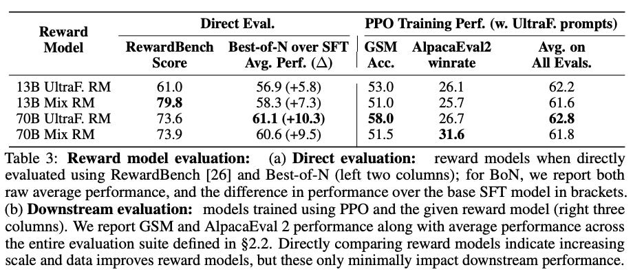
Put simply, using a bigger and better RM does not directly imply that our LLM will be better when this RM is used for RL finetuning. In fact, we even see a performance regression in some domains when using larger RMs in [13]. Such findings make the evaluation of RMs very complicated—just measuring the accuracy of an RM does not help us to understand how useful it will be.
RewardBench 2: Advancing Reward Model Evaluation [2]

The recently-proposed RewardBench 2 [2]6 aims to make improvements over the initial RewardBench so that evaluating RMs is more useful and informative. This benchmark contains new data that covers a wider scope of skills that LLMs may possess, and RMs score ~20 points lower on this benchmark on average—it is a much more challenging benchmark. Despite still using an accuracy-based approach for evaluating RMs, RewardBench 2 has a clear correlation with downstream RM usage (e.g., for Best-of-N sampling) and provides useful lessons for determining whether a given RM will be effective when used for RL finetuning.
Measuring RM performance. Instead of measuring the accuracy of the RM in differentiating between a chosen and rejected response, RewardBench 2 has four possible responses for each prompt—one chosen and three rejected. Among these responses, the RM must score the chosen response higher than all rejected responses; see below. This best-of-4 approach, which is still accuracy-based like the initial RewardBench, is more challenging and brings the performance of even strong RMs closer to that of the random baseline (i.e., 25% accuracy).

Additionally, RewardBench 2 goes beyond accuracy-based evaluation by measuring LLM performance when:
A certain RM is used for Best-of-N sampling.
A certain RM is used for RL training.
As a result of this extended evaluation, we can both understand the quality of an RM, as well as observe the impact of this quality on downstream performance when used for inference-time scaling and RL training. Compared to alternative benchmarks, this evaluation process is quite comprehensive; see below.

Data composition. RewardBench 2 focuses upon six different domains or capabilities when evaluating an RM. Three of these domains—focus, math and safety—overlap with existing benchmarks, while the three others—factuality, precise instruction following and ties (i.e., testing the RM’s ability to handle equally-valid answers)—present completely new challenges for RMs.
“The benchmark was created with a majority of previously unused human prompts from the WildChat pipeline with extensive manual, programmatic, and LM-based filtering techniques.” - from [2]
RewardBench 2 uses unseen and human-written prompts, largely sampled from WildChat—a dataset of ChatGPT logs collected from real-world users. Using unseen prompts is important due to the risk of data contamination. If our data is contaminated7, the RM benchmark will be highly correlated with downstream performance due to the same data being used for both evaluations. To ensure correlation is legitimate, we must decontaminate the data and avoid leakage.
To accomplish this goal, authors in [2] adopt a multi-stage data curation pipeline that involves:
Sourcing unseen, human-written prompts from WildChat.
Identifying the domain and quality of each prompt using manual inspection and classifiers; e.g., QuRater and domain classifiers.
Performing extensive data decontamination to ensure virtually zero overlap with downstream evaluation datasets.
Manually selecting the best prompts from those remaining.
Sampling completions for each of the prompts from diverse sources that accurately reflect the capabilities of recent LLMs.
Filtering completions based on correctness using a variety of signals; e.g., LLM-as-a-Judge, automatic verifiers, majority voting and more.
Details of the final dataset created for RewardBench 2 and how each component of this dataset is created are summarized below. To derive the final benchmark score, we take an unweighted average of an RM’s performance8 in each domain.

RewardBench 2 performance. RewardBench 2 is used to evaluate >100 different RMs in [2]. The performance of the top-20 models is provided below. In addition to scores being lower on this new benchmark, we see that foundation model-based (e.g., Gemini and Claude) LLM-as-a-Judge models perform very well. This observation—though in line with the improving capabilities of foundation models—is in stark contrast to observations on the initial RewardBench, where LLM-as-a-Judge models performed consistently worse than classifier-based RMs.

Authors in [2] also train a variety of their own RMs using various base models and hyperparameter settings, finding that the base model used to initialize the RM clearly impacts the RM—skills present in the base model carry over to the RM. Factors like the model family, training data mixture, style of training used or the stage of post-training from which the RM is initialized clearly influence the performance of the RM across domains. Additionally, authors in [2] find that training the RM for two epochs—instead of the usual one epoch—can be beneficial.
Downstream performance. Finally, the analysis of RMs in [2] is extended to consider inference-time scaling and RL training. Unsurprisingly, performance on RewardBench 2 is highly correlated with Best-of-N sampling—accurate reward models are capable of identifying the best completions within a candidate set.
Although correlation of RewardBench 2 with downstream performance is less clear, authors in [2] do identify one key factor that influences the success of an RM when used for RL training: whether the RM and the policy being trained are derived from the same model lineage. In other words, we see the following:
High scores on RM benchmarks are necessary (but not sufficient) for high downstream performance with RL training—downstream performance quickly saturates with improving RM quality9.
A misalignment between the policy model for RL training and the RM’s base model—or between the distribution of prompts used for RL training versus training the RM—causes a huge drop in downstream performance.
As a result of these findings, authors in [2] conclude their work by leaving us with a final recommendation for training RMs summarized in the below quote.
“These findings warrant caution when using reward model evaluation benchmarks: While the benchmark can be used as a guide for picking a reward model off-the-shelf to be used in some settings like best-of-N sampling… for policy-gradient algorithms like PPO, the results of the benchmark should be considered in the context of one’s training setup. Instead of simply taking the top model on RewardBench 2, we show that one should take the recipe for that model and integrate it into their specific workflow rather than the checkpoint itself.” - from [2]
Conclusion
Reward models are among the most powerful and flexible tools in LLM research. As we have learned, various styles of RMs exist beyond the standard classifier-based RM, and creating an effective RM is the result of countless practical considerations. Additionally, the correct choices for creating an RM are application-dependent; e.g., Best-of-N sampling versus RL finetuning. In this overview, we have built a foundational understanding of RMs, ranging from basic statistical models like Bradley-Terry to training large-scale LLM-based RMs. As more focus is dedicated to large-scale RL training for LLMs, research on RMs will rapidly advance and play an increasingly pivotal role in AI.
New to the newsletter?
Hi! I’m Cameron R. Wolfe, Deep Learning Ph.D. and Senior Research Scientist at Netflix. This is the Deep (Learning) Focus newsletter, where I help readers better understand important topics in AI research. The newsletter will always be free and open to read. If you like the newsletter, please subscribe, consider a paid subscription, share it, or follow me on X and LinkedIn!
Bibliography
[1] Lambert, Nathan, et al. "Rewardbench: Evaluating reward models for language modeling." arXiv preprint arXiv:2403.13787 (2024).
[2] Malik, Saumya, et al. "RewardBench 2: Advancing Reward Model Evaluation." arXiv preprint arXiv:2506.01937 (2025).
[3] Ouyang, Long, et al. "Training language models to follow instructions with human feedback." Advances in neural information processing systems 35 (2022): 27730-27744.
[4] Lambert, Nathan, et al. "T\" ulu 3: Pushing frontiers in open language model post-training." arXiv preprint arXiv:2411.15124 (2024).
[5] OpenAI et al. “Learning to Reason with LLMs.” https://openai.com/index/learning-to-reason-with-llms/ (2024).
[6] Rafailov, Rafael, et al. "Direct preference optimization: Your language model is secretly a reward model." Advances in Neural Information Processing Systems 36 (2023): 53728-53741.
[7] Guo, Daya, et al. "Deepseek-r1: Incentivizing reasoning capability in llms via reinforcement learning." arXiv preprint arXiv:2501.12948 (2025).
[8] Bai, Yuntao, et al. "Training a helpful and harmless assistant with reinforcement learning from human feedback." arXiv preprint arXiv:2204.05862 (2022).
[9] Zheng, Lianmin, et al. "Judging llm-as-a-judge with mt-bench and chatbot arena." Advances in Neural Information Processing Systems 36 (2023): 46595-46623.
[10] Bai, Yuntao, et al. "Constitutional ai: Harmlessness from ai feedback." arXiv preprint arXiv:2212.08073 (2022).
[11] Zheng, Lianmin, et al. "Judging llm-as-a-judge with mt-bench and chatbot arena." Advances in Neural Information Processing Systems 36 (2023): 46595-46623.
[12] Cobbe, Karl, et al. "Training verifiers to solve math word problems." arXiv preprint arXiv:2110.14168 (2021).
[13] Ivison, Hamish, et al. "Unpacking dpo and ppo: Disentangling best practices for learning from preference feedback." Advances in neural information processing systems 37 (2024): 36602-36633.
[14] Stiennon, Nisan, et al. "Learning to summarize with human feedback." Advances in neural information processing systems 33 (2020): 3008-3021.
Sometimes, we may have more than two candidate completions per prompt. In this case, preferences are captured by ranking completions in terms of their preference. However, binary preference data is more commonly used in recent research.
Here, we use the term policy to refer to an LLM that we are currently training. This is standard terminology used within reinforcement learning; see here.
In practice, these sequences will be both the prompt and the completion for all chosen and rejected sequences. Here, we just have flat textual sequences with no clear prompt or completion structure for simplicity.
At the time of writing, Llama-3 was the best open-source model that was available.
This benchmarks comes with data, a leaderboard, and an extensive technical report!
Data contamination refers to the idea of data being present in our training set that will later be used to evaluate the same model.
Performance is measured in terms of accuracy for all domains except ties, where we check for the correct margin between correct and incorrect examples.
This is in line with results in [13], where we see that RMs of various strengths all perform relatively well when used for RL training.
A little touch but seeing you do thjis--
chosen_seqs = [
"I love deep (learning) focus!",
"Cameron is great at explaining stuff",
"AGI is coming very soon...",
]
# Rejected prompt-response sequences
rejected_seqs = [
"I'm not a fan of deep (learning) focus",
"Cameron doesn't know what he's talking about",
"AGI is fake and LLMs can't reason!",
]
made me so happy. t's very cool to see you inject more personality here
Bewn in my inbox, glad I finally had a chance to read start to finish! Really insightful!