Group Relative Policy Optimization (GRPO)

How the algorithm that teaches LLMs to reason actually works...

(from [1, 19])

Reinforcement learning (RL) has always played a pivotal role in research on large language models (LLMs), beginning with its use for aligning LLMs to human preferences. More recently, researchers have heavily focused on using RL training to improve LLM reasoning performance. This line of research has led to a rapid expansion of LLM capabilities over the last few years. The objective of RL training (e.g., alignment or reasoning) has changed over time, along with the RL optimizers that are used to achieve these goals. Most early work on RL for LLMs used Proximal Policy Optimization (PPO) as the default RL optimizer, but recent reasoning research relies upon Group Relative Policy Optimization (GRPO).

This overview will provide a deep dive into GRPO, where it comes from, how it works, and the role it has played in creating better large reasoning models (LRMs). As we will learn, RL training—even with GRPO—is a complex process that presents a seemingly endless frontier of open research questions. However, GRPO is a refreshingly simple—and effective—algorithm that is more efficient and approachable than its predecessors. These characteristics allow GRPO to democratize RL research and, in turn, accelerate progress on both:

1. Building a better collective understanding of RL for LLMs.

2. Training more powerful reasoning models.

Basics of RL. We will not discuss the basics of RL (e.g., terminology, problem setup, or policy gradients) in this overview. To gain a more comprehensive grasp of the foundational ideas in RL that are useful for understanding GRPO, please see the following excerpts from prior articles:

• RL Problem Setup & Terminology [link]

• Different RL Formulations for LLMs [link]

• Policy Gradient Basics [link]

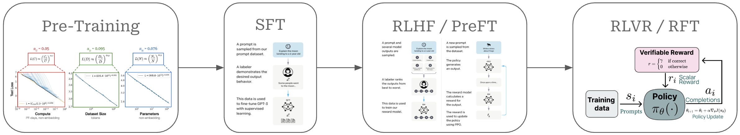
Reinforcement Learning (RL) for LLMs

(from [19])

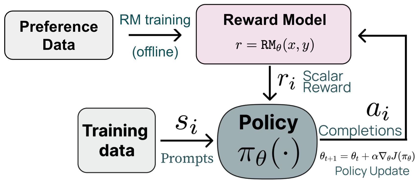
To begin our discussion, we will cover some preliminary details on reasoning models and reinforcement learning (RL). Specifically, we will first discuss the two most common RL frameworks used for training LLMs (depicted above):

1. Reinforcement Learning from Human Feedback (RLHF) trains the LLM using RL with rewards derived from a reward model trained on human preferences.

2. Reinforcement Learning with Verifiable Rewards (RLVR) trains the LLM using RL with rewards derived from rule-based or deterministic verifiers.

After this discussion, we will provide further details on large reasoning models (LRMs), which are LLMs that have been extensively trained (via RLVR) to hone their complex reasoning capabilities. This discussion is relevant to GRPO, as it is currently the most common RL optimizer—at least for open LLMs—to use for training LRMs with RLVR. In fact, GRPO gained popularity primarily through its use in training open reasoning models like DeepSeek-R1 [8]!

General RL setup. The main difference between RLHF and RLVR lies in how we assign rewards—RLHF uses a learned reward model, while RLVR uses verifiable (or rules-based) rewards. Despite this difference, these are both online RL algorithms that follow a similar training framework; see below.

General framework for online RL

We first sample a batch of prompts and generate a completion—or multiple completions—for each prompt in the batch using our current policy. A reward is computed for each completion, which can then be used to derive a policy update using our RL optimizer of choice—this is where GRPO comes in! GRPO is a generic RL optimizer that is used to compute the policy update (i.e., the update to our LLM’s weights) during RL training. GRPO is usually used for RLVR, while PPO is usually used for RLHF. However, RL optimizers are generic, and technically any RL optimizer can be used to derive the policy update in these frameworks.

Reinforcement Learning from Human Feedback (RLHF)

(from [16])

The first form of RL training to be popularized in the LLM domain was Reinforcement Learning from Human Feedback (RLHF). Early post-ChatGPT LLMs were almost always post-trained using the following three-step alignment procedure (depicted above), as proposed by InstructGPT [16]:

1. Supervised finetuning (SFT)—a.k.a. instruction finetuning (IFT)—trains the model using next-token prediction over examples of good completions.

2. A reward model is trained over a human preference dataset.

3. Reinforcement learning (RL)—usually with PPO—is used to finetune the LLM with the reward model as the reward signal.

The second and third steps of this procedure are collectively referred to as RLHF. This framework actually involves two training procedures: a supervised learning phase for the reward model and an RL training phase for the LLM.

(from [17])

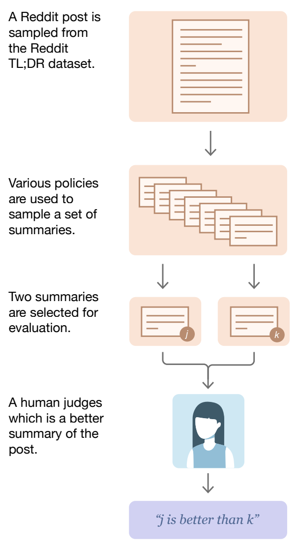
Preference data is the foundation of RLHF. Each element of a preference dataset consists of a prompt, two completions to that prompt, and a preference label—assigned either by human or an AI or LLM judge—indicating which completion is preferred to the other. Specifying an explicit reward for an LLM is very difficult—how do we reliably determine whether a completion is “good” or not when the model has so many diverse capabilities? Instead of answering this question directly, we can instead collect preference data, which captures preferred model behavior via examples of ranked model responses for a particular prompt. A typical interface for collecting preference annotations can be seen in the figure below.

(from [18])

Choosing the better model response is relatively intuitive, though it does require detailed guidelines on alignment criteria to ensure data quality. Preference data is used extensively in LLM post-training because:

1. We can use it to train our model to produce human-preferable responses.

2. We just have to select a preferred response (rather than define an explicit reward signal or manually write responses from scratch).

After collecting sufficient preference data, we have many examples of preferred model behavior that can be used to align our LLM to human (or AI-generated) preferences. We can directly train an LLM on this preference data using a direct alignment algorithm like Direct Preference Optimization (DPO), but we usually incorporate this data into RL by first using it to train a reward model.

Reward model architecture

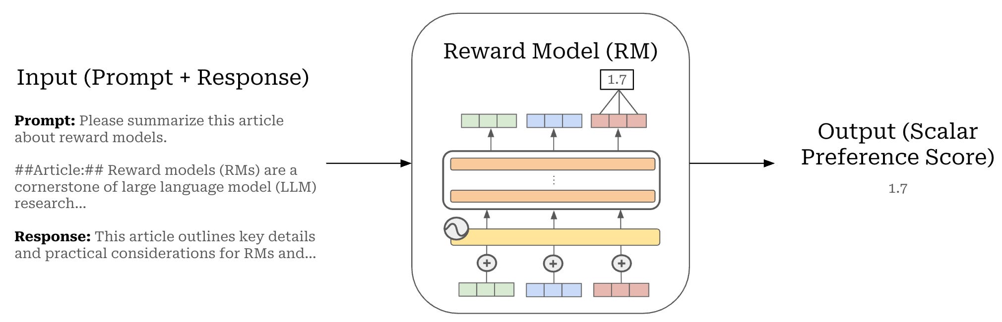
Reward models. A reward model is a specialized LLM—usually a copy of the LLM we are training with an added regression head (depicted above)—that is finetuned to predict a human preference score given a prompt and candidate completion as input. Specifically, the reward model is finetuned on our preference data using a ranking loss function that is derived from the Bradley-Terry model; see below.

Reward model loss function

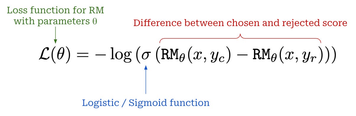
Put simply, this loss function teaches the reward model to assign a higher score to the preferred response in a preference pair relative to the rejected response. The reward model is trained over paired preference data, but we see above that the model outputs an individual preference score for each completion in the pair. More details on reward models can be found in the overview below.

Reward Models

Input and output structure of a reward model

PPO & RLHF. Once the reward model has been trained over the preference data using this loss, the model learns how to assign a preference score to each model completion; see above. We can directly use this reward model as a reward signal for RL training. For RLHF, we usually use Proximal Policy Optimization (PPO) [12], which we will cover later in more detail, as the underlying RL optimizer.

“Reward models broadly have been used extensively in reinforcement learning research as a proxy for environment rewards.” - RLHF book

Our LLM is indirectly trained on human feedback via the reward model. We begin with a preference dataset, which captures human preference via concrete examples of ranked model outputs. This data is used to train a reward model that can assign accurate preference scores to arbitrary outputs from the LLM. During training with RL, we generate new outputs—or on-policy samples—from our LLM and score them with the reward model. These scores serve as the reward signal, and our RL optimizer updates the model’s weights to maximize rewards. Since the reward here is the output of our reward model, we are maximizing preference scores. In this way, the RL training process guides the LLM to produce outputs that align with human preferences, as estimated by the reward model.

Schematic depiction of RLHF (from [19])

Impact of RLHF. The ability to align an LLM to human preferences is a hugely impactful technology that catalyzed the popular use of LLMs. If we think about the differences between well-known LLMs like ChatGPT and their less widely-recognized predecessors, one of the key enhancements made to ChatGPT was the use of more sophisticated post-training. Specifically, ChatGPT was extensively aligned via SFT and RLHF, which significantly improved the model’s helpfulness. In this way, RL research—and RLHF in particular—played a pivotal role in creating the impressive and capable LLMs that we have today.

Reinforcement Learning from Verifiable Rewards (RLVR)

The reward in RLHF is derived from a reward model. This reward model requires its own training pipeline and validation, which adds costs and complexity to the RL training process. Our policy could also suffer from reward hacking, even when using a high-quality reward model. The policy explores the space of possible completions during RL to maximize rewards. If we continue running RL for long enough, however, the model may learn to maximize rewards via an exploit or hack in our reward model, rather than by generating better completions.

“Reinforcement Learning with Verifiable Rewards (RLVR) can be seen as a simplified form of… RL with execution feedback, in which we simply use answer matching or constraint verification as a binary signal to train the model.” - from [13]

Put simply, reward models—despite their incredible impact through RLHF—have downsides. Reinforcement Learning from Verifiable Rewards (RLVR) chooses to avoid reward models, instead deriving rewards from manually verifiable and deterministic sources (e.g., rules or heuristics). Using verifiable rewards instead of neural reward models reduces the risk of reward hacking and makes extensive, large-scale RL training more feasible by making rewards harder to game.

Schematic depiction of RLVR (from [19])

Verifiable domains and rewards. To train an LLM with RLVR, we must select a domain that is verifiable in nature; e.g., math or coding. In other words, we need to create a dataset that has either i) a known ground truth answer or ii) some rule-based technique that can be used to verify the correctness of an answer for each prompt in our dataset. For coding, we can create a sandbox for running LLM-generated code and use test cases to assess correctness. Similarly, we can evaluate math problems by performing basic string matching between the answer predicted by the LLM and a ground-truth answer for a problem; see below.

Verifying a problem with exact string matching

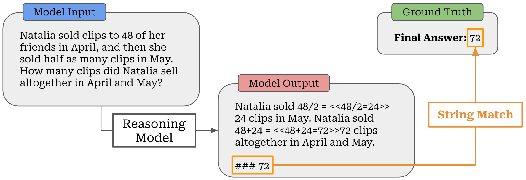
Usually, we must instruct the LLM to format its output such that the final answer can be easily parsed. Even then, however, string matching is not always sufficient for evaluating correctness. In many cases, we can benefit from crafting validation logic that is more robust (e.g., asking an LLM to tell us if two answers are the same [20]) and that captures variations in format for similar or identical outputs.

“Math verification is determined by an LLM judge given the ground truth solution and DeepSeek-R1 solution attempt. We found that using an LLM judge instead of a stricter parsing engine (Math-Verify) for verification during data generation results in a higher yield and leads to higher performing downstream models.” - from [20]

Applications of RLVR. Beyond substituting a reward model with verifiable rewards, the RL component of RLVR is unchanged. However, RLHF and RLVR differ in their purpose and application:

1. RLHF is usually implemented with PPO as the underlying RL optimizer, while GRPO is the most common RL optimizer for RLVR.

2. RLHF focuses on LLM alignment with preference feedback, while RLVR is used to improve the complex reasoning capabilities of an LLM.

Most recent research on LLMs and RL is heavily focused on creating LLMs with better reasoning capabilities, known as large reasoning models (LRMs). The training process for LRMs is centered around performing RLVR on domains like math and coding. In these training setups, GRPO is the most commonly used RL optimizer—at least for open LLMs. As we will see in this overview, several notable results have already been achieved from using RLVR (with GRPO) to train LRMs. However, this area of research is still incredibly active and dynamic. Examples of popular topics being explored in this area include:

• Tweaking or improving GRPO

• Scaling the RLVR training process

• Expanding to non-verifiable domains via rubrics

• Using curriculum learning to improve RLVR

• Combining verifiable and non-verifiable rewards

Large Reasoning Models (LRMs)

As mentioned before, RLVR and GRPO can be used to improve the reasoning capabilities of LLMs on verifiable tasks, and research on this topic has led to the creation of large reasoning models (LRMs). The key distinction between an LRM and a standard LLM is the ability to dynamically “think” about a prompt prior to providing a final output. By increasing the length of the thinking process, these LRMs can use inference-time scaling—or simply spend more compute on generating a completion—to improve their performance.

“We’ve developed a new series of AI models designed to spend more time thinking before they respond.” - from [4]

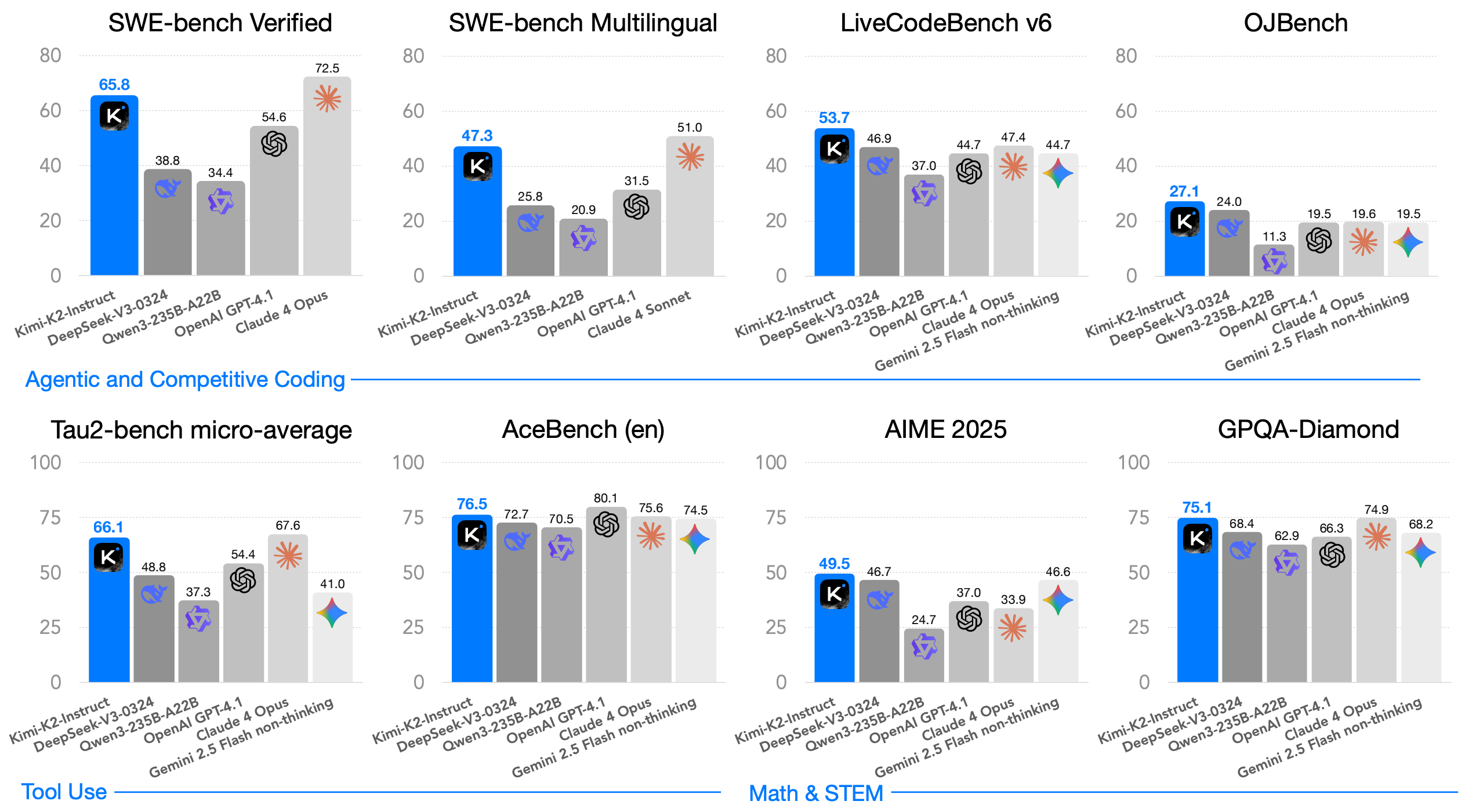
One of the first such models to be released was OpenAI’s o1-preview, which was predated by a long series of rumors about OpenAI developing a new series of LLMs with complex reasoning capabilities. This model has since been followed by a massive number of new closed (e.g., o3 / o4 or Gemini 3) and open (Qwen-3, DeepSeek-R1, and Olmo-3) LRMs as the research community continues to iterate on these ideas. Interestingly, the popularization of LRMs has also led to a proliferation of open models—mostly proposed after DeepSeek-R1 [8], which we will discuss later on. Recent open LRM releases like Kimi-K2 [14] have even started to match or exceed the performance of closed models; see below.

(from [14])

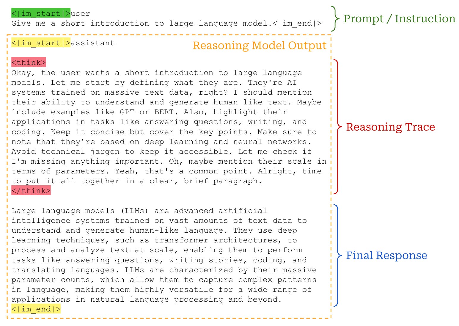
How do LRMs work? LRMs and LLMs are identical architecturally¹. They are both based upon decoder-only transformers, potentially with a Mixture-of-Experts (MoE) architecture. Their main difference lies in how they generate output. At a high level, LRMs operate by allowing the model to “think” prior to producing a final output. This thinking process occurs in the form of a long, free-text chain-of-thought (CoT)—also called a rationale or reasoning trajectory—that is generated by the LLM. Most closed LRMs hide this reasoning trajectory from the end-user for safety purposes². The user sees only the model’s final output and (optionally) a truncated summary of the reasoning process.

(from [9])

For open LRMs, we can observe the model’s reasoning process and final output. Concretely, LRMs use special tokens to separate their reasoning process from their actual output. The reasoning trajectory is generated first and is wrapped between <think> tokens. The model ends its reasoning process with a </think> token, then proceeds to generate a final response; see below.

Concrete example of LRM output in Qwen-3 prompt format

Reasoning trajectories. If we look at some examples of reasoning trajectories from open or closed LRMs, we will notice that these models exhibit sophisticated reasoning behaviors in their long CoT:

• Thinking through each part of a complex problem.

• Decomposing complex problems into smaller, solvable parts.

• Critiquing solutions and finding errors.

• Exploring many alternative solutions.

In many ways, the model is performing a complex, text-based search process to find a viable solution to a prompt. Such behavior goes beyond any previously-observed behavior with standard LLMs and chain of thought prompting. With this in mind, we might begin to wonder: How does the model learn how to do this?

LRM training. LRMs also differ from standard LLMs in their training methodology. Though exact post-training details may vary significantly between models, both LLMs and LRMs undergo similar pretraining and alignment phases that consist of supervised finetuning (SFT) and RLHF.

However, LRMs extend this standard training process by performing large-scale RLVR on verifiable domains like math and code. Because verifiable reward signals are less prone to reward hacking, we can perform larger-scale RL training (i.e., by running the training process longer) with less risk of training collapse. Several works [8, 9] have shown that LRMs obey a predictable scaling law with respect to the amount of compute used during RL training, meaning that we can achieve better performance by increasing the number of RL training steps.

“We do not apply the outcome or process neural reward model in developing DeepSeek-R1-Zero, because we find that the neural reward model may suffer from reward hacking in the large-scale reinforcement learning process.” - from [8]

The complex reasoning behaviors of an LRM are not directly encoded into the model in any way. Rather, this behavior naturally emerges from large-scale RL training. The LRM undergoes an RL-powered self-evolution as it attempts to solve problems and is rewarded for finding correct solutions. From this process, the model learns to properly leverage its reasoning trajectory. We will continue discussing the details of RL training for LRMs throughout the remainder of this post, but the key idea here is to:

• Create the correct incentives for RL training—usually a deterministic or rule-based reward signal that is at low risk for reward hacking.

• Run large-scale RL training with these reliable reward signals.

• Allow sophisticated model behavior to naturally emerge.

Powerful LRMs are a product of large-scale RL with the correct incentives, but there are many practical details involved in properly incentivizing and scaling the RL training process—this is still a very active area of research [15].

Are LRMs a silver bullet? Given the impressive performance of LRMs in complex reasoning domains, we might naively believe that LRMs will outperform standard LLMs at all tasks. However, the story is not this simple—LRMs are not always the best tool to use. Because the training process for LRMs is focused on verifiable domains like math and code, their performance may be biased towards these domains—and away from non-verifiable domains like creative writing.

“Reasoning models are designed to be good at complex tasks such as solving puzzles, advanced math problems, and challenging coding tasks. However, they are not necessary for simpler tasks like summarization, translation, or knowledge-based question answering. In fact, using reasoning models for everything can be inefficient and expensive. For instance, reasoning models are typically more expensive to use, more verbose, and sometimes more prone to errors due to overthinking.” - Sebastian Raschka

LRMs may also have deficiencies in alignment (e.g., instruction following or reading-friendly formatting) relative to standard LLMs. However, most of these issues are being solved as we continue to study the interplay between RLHF and RLVR. We should use LRMs for the domains in which they excel but be sure to test their performance in non-verifiable domains. Using a standard LLM may be sufficient—or better—and is usually more efficient in terms of inference-time compute.

GRPO from Idea to Implementation

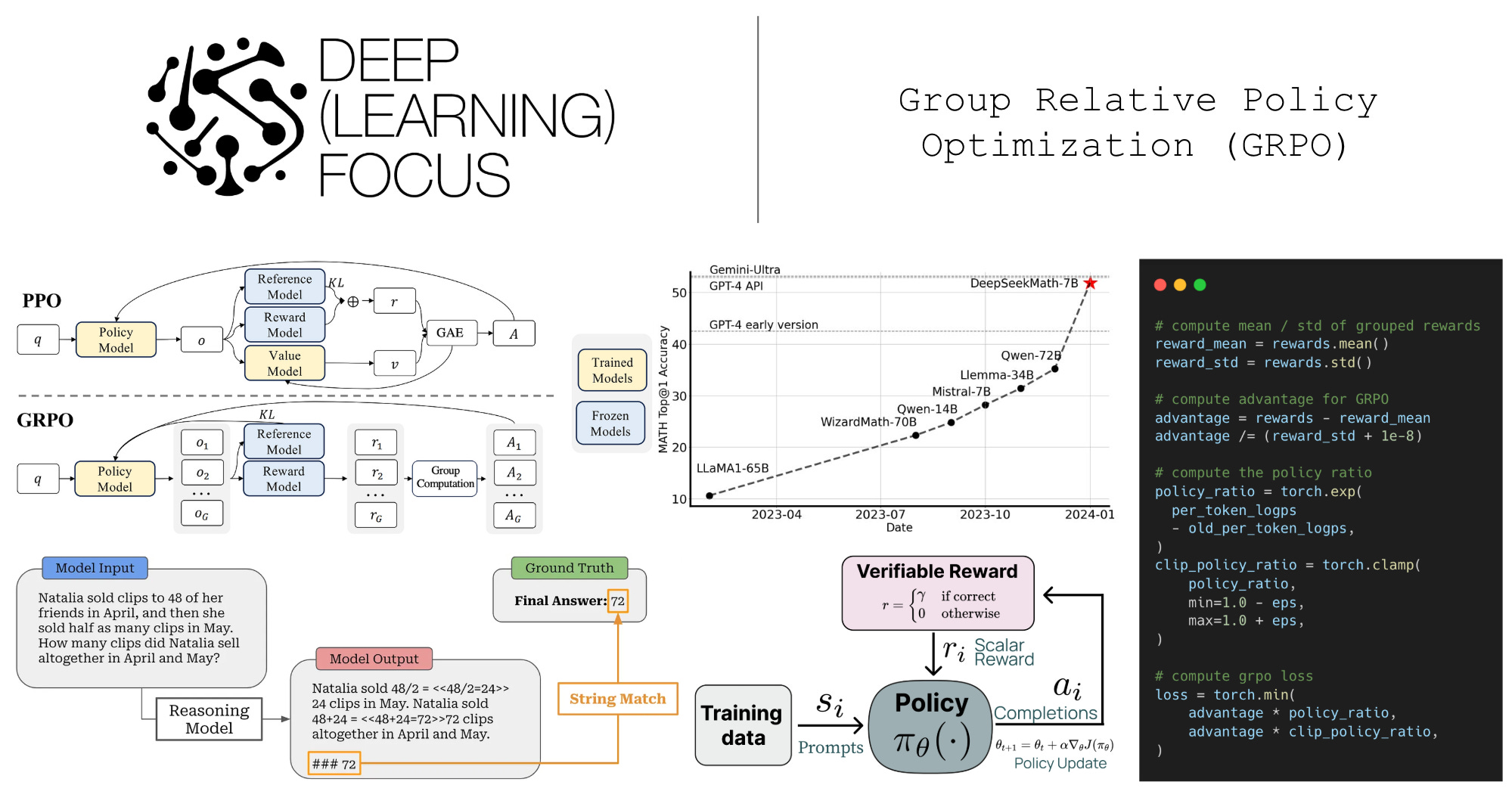
Now that we understand how RL is used to train LLMs (and LRMs), we will take a deeper look at common RL optimizers used to derive policy updates for RLHF and RLVR. To begin, we will learn about Proximal Policy Optimization (PPO) [12] before moving on to the main topic of this overview—Group Relative Policy Optimization (GRPO) [1]. GRPO is inspired by PPO and shares some of its core ideas. However, GRPO also goes beyond PPO by making several changes to simplify the algorithm while maintaining effectiveness for LLM training.

Proximal Policy Optimization (PPO) [12]

GRPO is heavily based upon the Proximal Policy Optimization (PPO) algorithm [12]. PPO was used in seminal work on RLHF and, as a result, became the default RL optimizer in the LLM domain for some time. Only recently with the advent of LRMs have alternative algorithms like GRPO started to become popular.

(from [12])

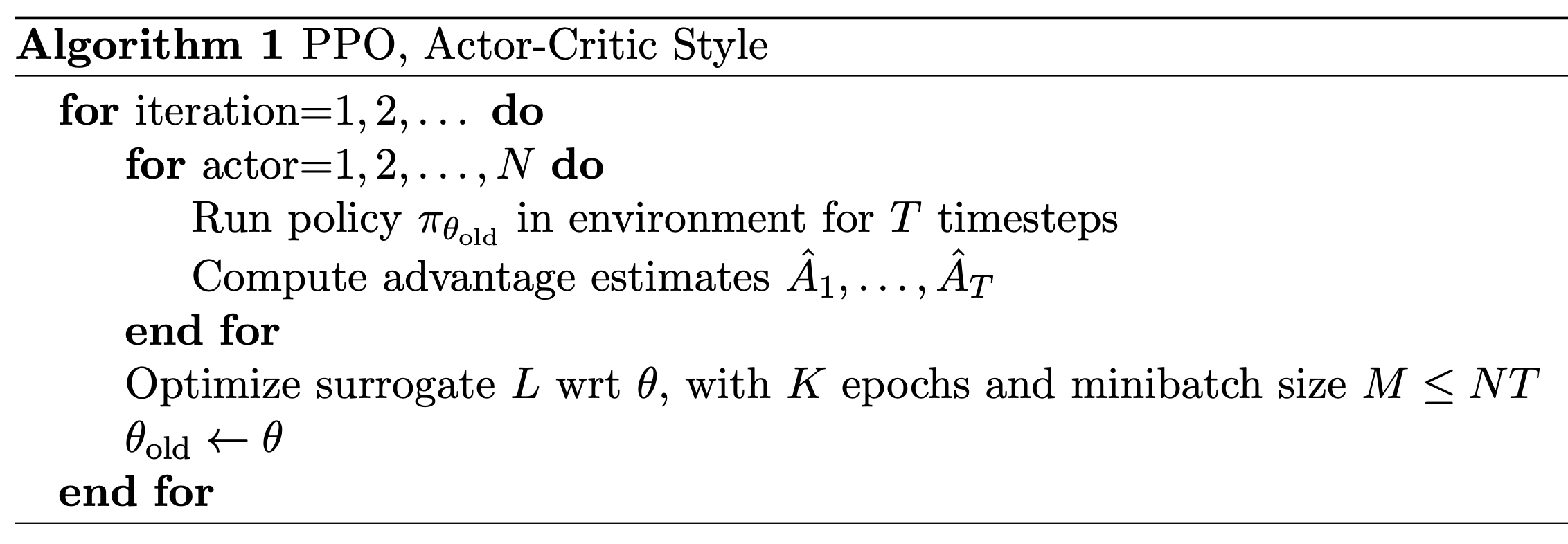
The structure of PPO is outlined above. As we can see, each training iteration of PPO performs the following sequence of steps:

1. Sample a diverse batch of prompts.

2. Generate a completion from the policy for each prompt.

3. Compute advantage estimates for each completion.

4. Perform several policy updates over this sampled data.

Surrogate objective. During PPO, we formulate a surrogate objective³ that is optimized with respect to the parameters of our policy. The PPO surrogate objective is based upon the policy ratio between the current policy and an old model (i.e., the policy as it existed before the first update in a training step). The policy ratio—also called the importance ratio—stabilizes the training process by comparing the new policy’s token probabilities to the old policy and applying a weight (or importance) to training that helps to avoid drastic changes; see below.

Policy or importance ratio

To derive the surrogate objective for PPO, we begin with an unclipped objective that resembles the surrogate objective used in Trust Region Policy Optimization (TRPO); see below. Additionally, we introduce a clipped version of this objective by applying a clipping mechanism to the policy ratio r_t(θ). Clipping forces the policy ratio to fall in the range [1 - ε, 1 + ε]. In other words, we avoid the policy ratio becoming too large or too small, ensuring that the token probabilities produced by the current and old policies remain relatively similar.

The PPO surrogate objective

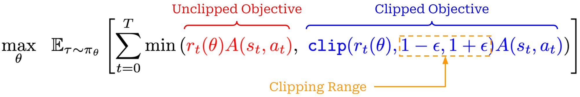
In PPO, the surrogate objective is simply the minimum of clipped and unclipped objectives, which makes it a pessimistic (lower bound) estimate for the unclipped objective. The behavior of the surrogate loss’ clipping mechanism changes depending on the sign of the advantage. The possible cases are shown below.

(from [12])

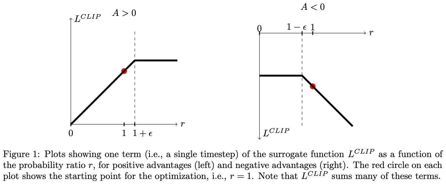
As we can see, taking the minimum of clipped and unclipped terms in the surrogate objective causes clipping to be applied in only one direction. The surrogate objective can be arbitrarily decreased by moving the policy ratio away from one, but clipping prevents the objective from being increased beyond a certain point by limiting the policy ratio. In this way, the clipping mechanism of PPO disincentivizes large policy ratios and, in turn, maintains a trust region by preventing large policy updates that could potentially damage our policy.

“We only ignore the change in probability ratio when it would make the objective improve, and we include it when it makes the objective worse.” - from [12]

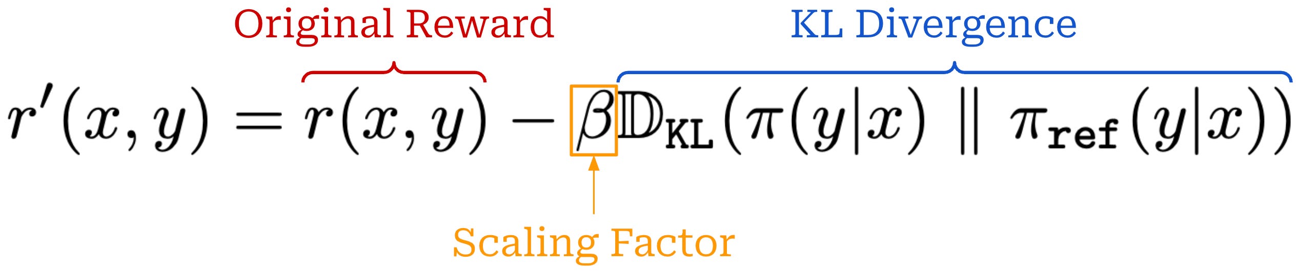
KL divergence. When training LLMs with PPO, we usually incorporate the KL divergence between the current policy and a reference policy—like the SFT model—into training. The KL divergence serves as a penalty that encourages similarity between the current and reference policies. We compute the KL divergence by comparing token distributions from the two LLMs for each token in a sequence. The easiest—and most common—way to approximate KL divergence [7] is via the difference in log probabilities between the policy and reference; see here.

\(\texttt{kl_div} = \texttt{policy_logprobs} - \texttt{ref_logprobs}\)

After the KL divergence has been computed, there are two primary ways that it can be incorporated into the RL training process:

1. By directly subtracting the KL divergence from the reward.

2. By adding the KL divergence to the loss function as a penalty term.

PPO adopts the former option by subtracting the KL divergence directly from the reward signal used in RL training as shown in the equation below.

Adding KL to the reward in PPO

Advantage estimation. The advantage function, a key part of PPO’s surrogate objective, is the difference between the action-value and value function: A(s, a) = Q(s, a) - V(s). The value function in PPO is estimated with a learned model called the value model or critic. This critic is usually a separate copy of our policy, or—for better parameter efficiency—an added value head that shares weights with the policy. The critic takes a completion as input and predicts expected cumulative reward on a per-token basis by using an architecture that is similar to that of a reward model (i.e., a transformer with a regression head)⁴; see below.

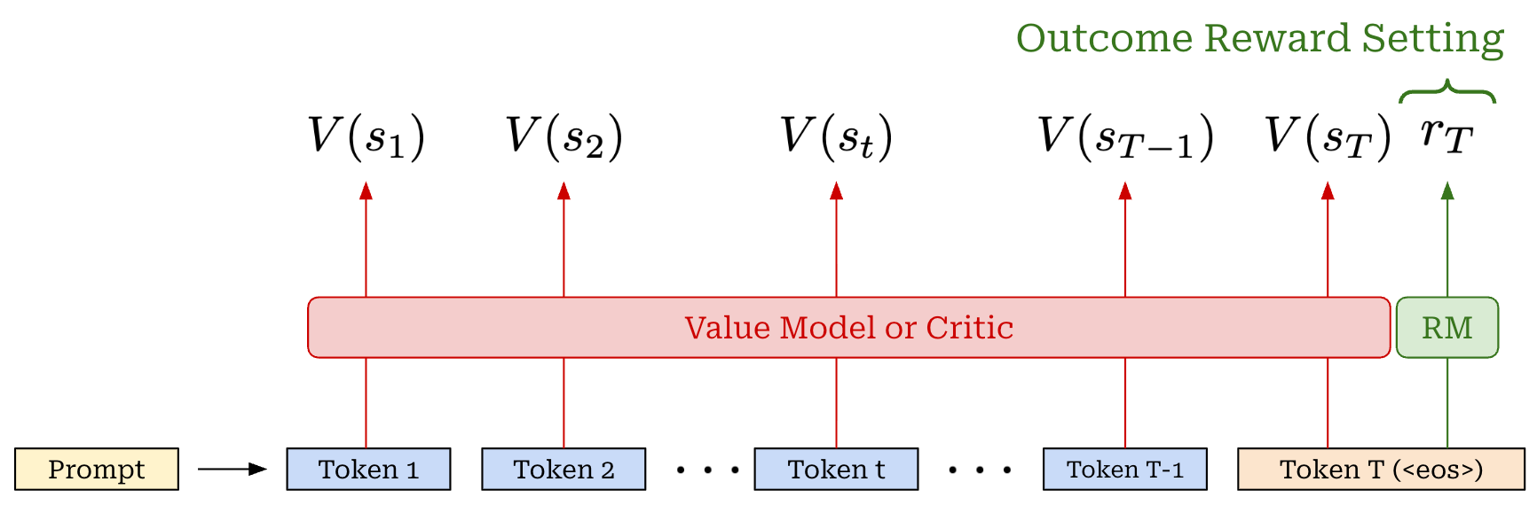
The value function is also on-policy, meaning it depends on the current parameters of our policy. Unlike reward models, which are fixed at the beginning of RL training, the critic is trained alongside the LLM in each policy update to ensure its predictions remain on-policy. This is known as an actor-critic setup. To handle this, we can add an extra mean-squared error (MSE) loss term—between the rewards predicted by the critic and actual rewards—to the surrogate loss for PPO.

The critic can be used to compute the advantage via Generalized Advantage Estimation (GAE) [13]. The details of GAE are beyond the scope of this post. We will only cover GAE at a high level, but a full explanation can be found here. GAE builds upon the concept of a temporal difference (TD) residual; see below.

The TD residual

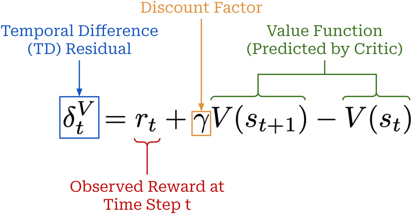
The TD residual uses per-token value predictions from the critic to form a one-step estimate of the advantage. Put simply, the TD residual is analyzing how much the reward changes after predicting a single token relative to the expected reward. However, the TD residual only uses a small amount of actual reward information (i.e., the reward at step t) to estimate the advantage, which causes the estimate to become biased⁵. To solve this issue, we can generalize the single-step TD residual to form a series of N-step advantage estimators; see below.

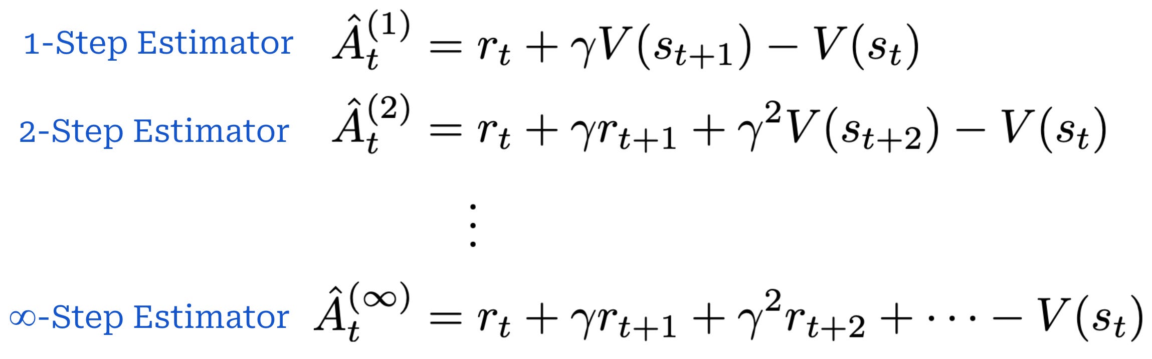
N-step advantage estimators

Similarly to the single-step TD residual, advantage estimators with lower values of N have low variance but high bias. As we increase the value of N, however, we are incorporating more exact reward information into the advantage estimate, thus lowering the bias (and, in turn, increasing variance). GAE tries to find a balance between these two ends of the spectrum by i) using all values of N and ii) taking an average of these advantage estimates. This is accomplished with the mixing parameter λ for GAE, as shown below.

GAE formulation

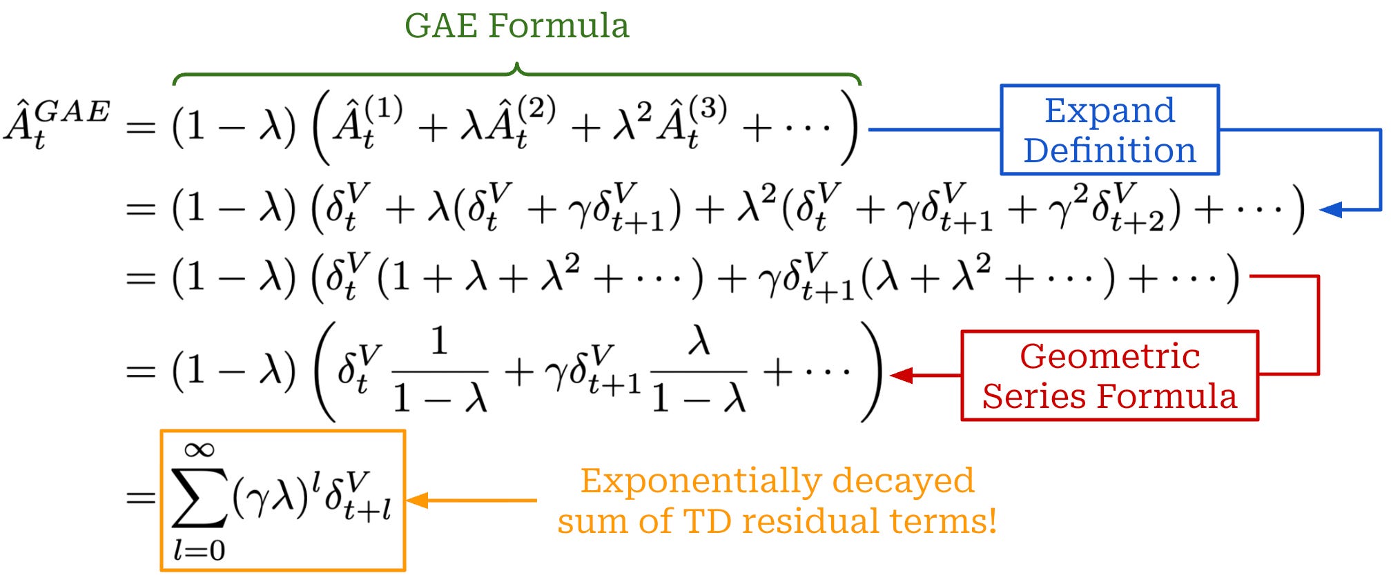
The value of λ ∈ [0, 1] controls the bias variance tradeoff. We can toggle the value of λ in GAE as needed to stabilize the training process⁶. For example, if training is unstable, we can decrease λ to yield lower variance policy updates.

Complexity of PPO. As we might infer from the above discussion, PPO is not a simple algorithm—there are many more details to be learned. For a more complete overview of PPO, please see the article linked below. However, we need to briefly discuss the key limitations of PPO to serve as motivation for GRPO.

There are a total of four models included in PPO’s training process: two that are being trained (i.e., the policy and the critic) and two that are used for inference (i.e., the reference and reward model). The fact that the critic must be trained in tandem with the policy complicates the training process, increases compute costs, and consumes a lot of memory. Plus, there are many additional nuances and settings that must be carefully tuned to arrive at a working PPO implementation (e.g., GAE, value model setup, reward model setup, clipping, and more).

“During RL training, the value function is treated as a baseline in the calculation of the advantage for variance reduction. In the LLM context, usually only the last token is assigned a reward score by the reward model, which may complicate the training of a value function that is accurate at each token.” - from [1]

Can we simplify PPO? Much of the complexity of PPO—though not all!—stems from estimating the per-token value function with the critic. Recent work has questioned the need for this critic, arguing that critic-free RL algorithms like REINFORCE can be used instead of PPO to train LLMs with no performance degradation. This argument stems from a few key observations:

• Avoiding high-variance policy updates—which is the key benefit of PPO and a limitation of simpler RL optimizers like REINFORCE—is less of a concern for LLMs because we are finetuning models that are extensively pretrained.

• LLMs are mostly trained using outcome rewards, which makes estimating advantage on a per-token basis unnecessary. How can we learn an accurate per-token value estimate from outcome rewards only? Modeling the advantage and reward on a completion level should be sufficient for LLMs in this case.

GRPO provides further empirical support for these claims in the LLM domain. Specifically, GRPO forgoes the critic and estimates advantage by averaging rewards for multiple completions to the same prompt. Each token in GRPO receives the same advantage estimate, rather than attempting to assign credit on a per-token basis from a sequence-level (outcome) reward signal.

Group Relative Policy Optimization (GRPO)

(from [1])

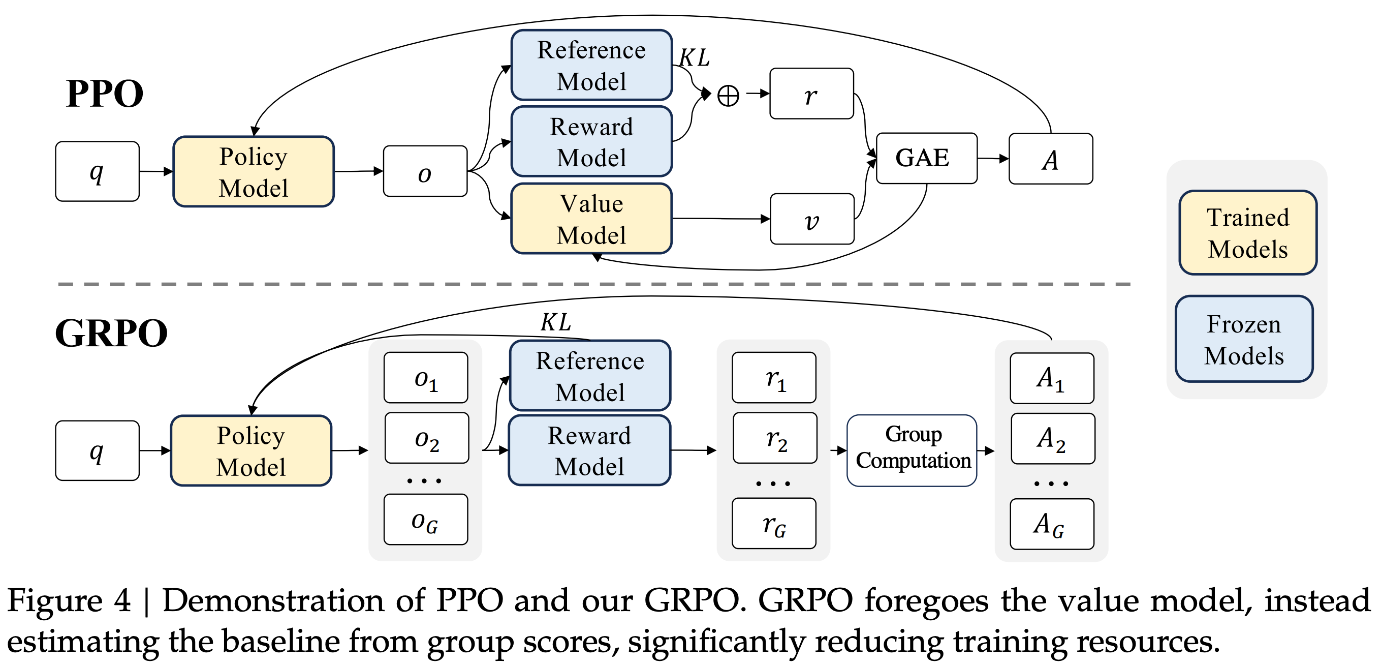
Group Relative Policy Optimization (GRPO) [1] builds upon PPO by proposing a simpler technique for estimating the advantage. In particular, GRPO estimates the advantage by sampling multiple completions—or a “group” of completions—for each prompt and using the rewards of these completions to form a baseline. This group-derived baseline replaces the value function, which allows GRPO to forgo training a critic. Avoiding the critic drastically reduces GRPO’s memory consumption and training complexity compared to PPO.

“We introduce the Group Relative Policy Optimization (GRPO), a variant of Proximal Policy Optimization (PPO). GRPO foregoes the critic model, instead estimating the baseline from group scores, significantly reducing training resources.” - from [1]

Advantage estimation in GRPO. Instead of using a learned value model, GRPO estimates the advantage by sampling multiple completions for each prompt in the batch and using the formulation shown below to compute the advantage.

Advantage computation in GRPO

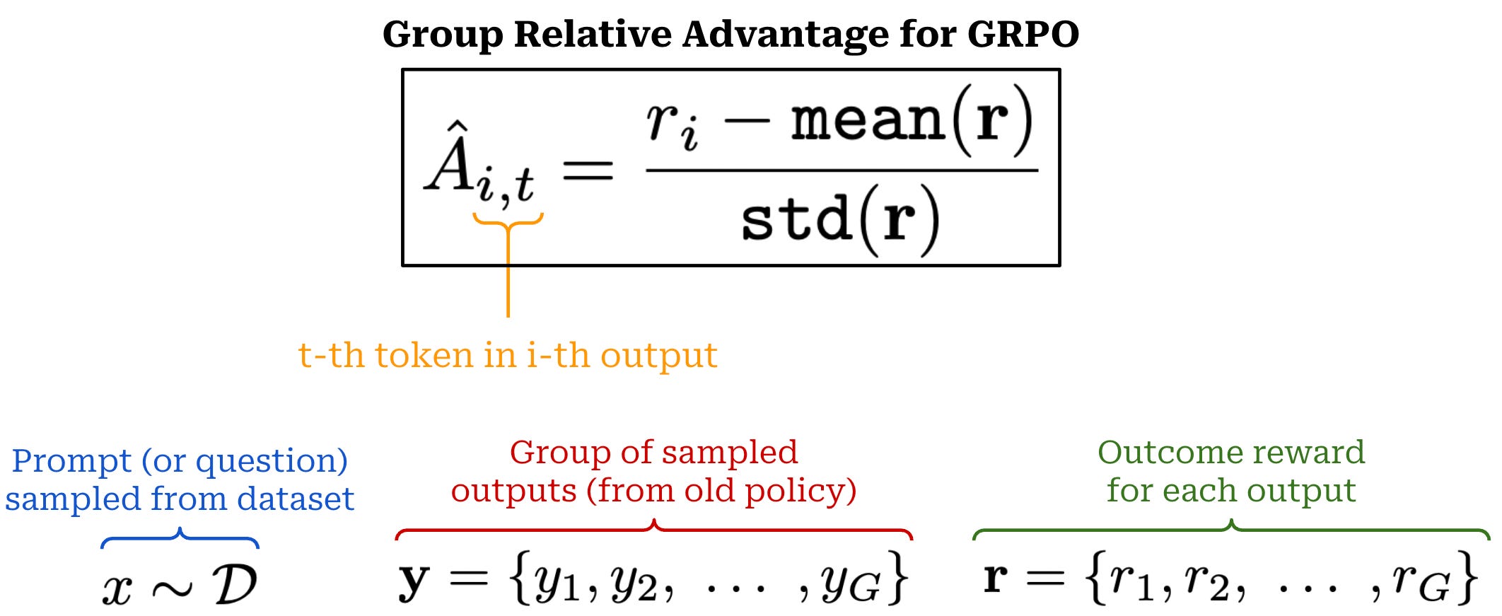
In GRPO, completions to the same prompt form a group, and we calculate the advantage relative to other rewards observed in the group—hence, the name “group relative” policy optimization! More specifically, the advantage for completion i is calculated by first subtracting the mean reward over the group from r_i, then dividing this difference by the standard deviation of rewards over the group. We are still assuming an MDP formulation in this discussion, but the formulation above assigns the same advantage to every token t in the sequence i.

“GRPO is often run with a far higher number of samples per prompt because the advantage is entirely about the relative value of a completion to its peers from that prompt.” - RLHF book

Because we compute the advantage in a relative manner (i.e., based on rewards in the group), the number of completions we sample per prompt must be high to obtain a stable policy gradient estimate. Unlike GRPO, PPO and REINFORCE typically sample a single completion per prompt. However, sampling multiple completions per prompt has been explored by prior RL optimizers like RLOO.

Surrogate loss. Despite estimating the advantage differently, GRPO uses a surrogate loss that is nearly identical to that of PPO. Both of these optimizers make use of the same clipping mechanism for the policy ratio; see below.

GRPO surrogate loss

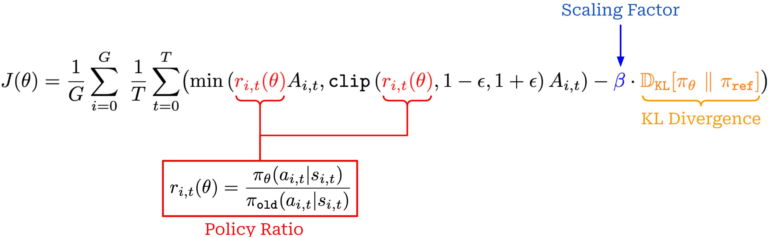
This expression assumes an MDP formulation and has been modified to explicitly aggregate the loss over multiple completions within a group. In contrast, we previously formulated the loss for PPO as an expectation over completions.

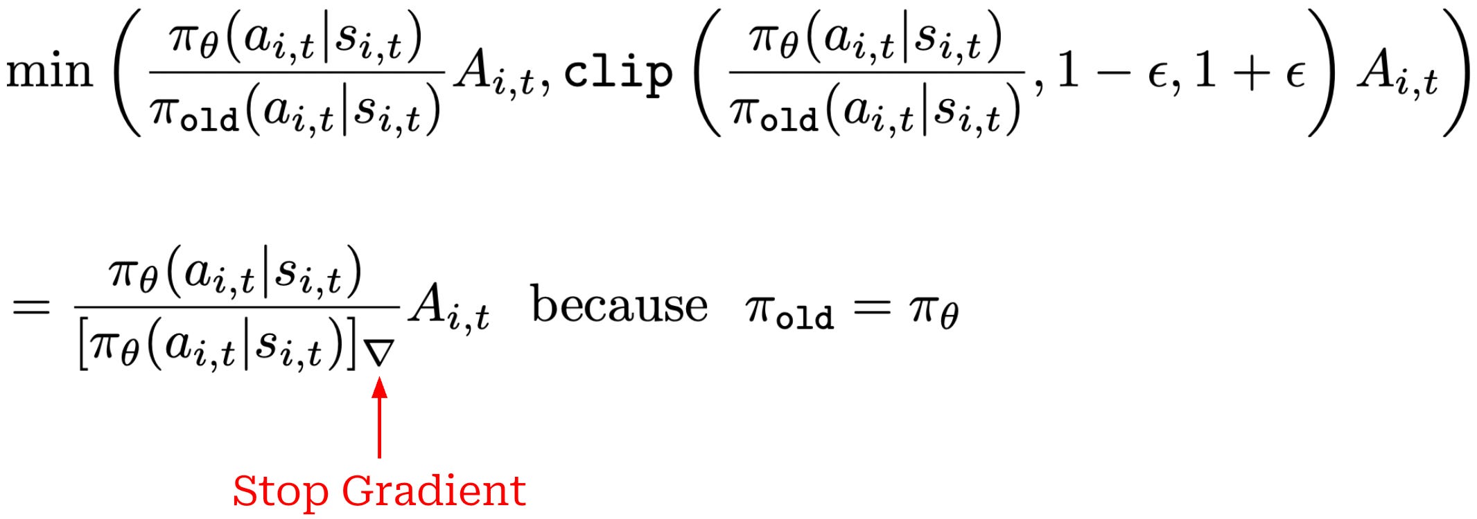
One key difference between PPO and GRPO is the KL divergence term being subtracted as a penalty term from the surrogate loss rather than incorporated into the per-token reward. Additionally, GRPO does not always perform multiple policy updates per batch of data. If we only perform a single policy update per batch, we have π_θ = π_old, which simplifies the clipped objective to the expression shown below⁷. See here for more discussion on this topic.

Simplification of the clipping term with a single update

Extension to process rewards. Most implementations of GRPO use outcome rewards, as this is the most common setting for an LLM. However, we can extend GRPO to handle process rewards (e.g., after each reasoning step) by:

1. Normalizing rewards based on the mean and standard deviation of all process rewards observed in the group.

2. Computing the advantage of each token as the sum of normalized rewards for following steps in the reasoning trajectory.

When using outcome rewards, each token is assigned the same advantage by GRPO, but this approach changes when using process rewards. The advantage is estimated for each token based on rewards observed in following steps of the trajectory, which changes depending on the position of a token. Additionally, we must now consider all rewards—including multiple rewards in each trajectory—when computing the mean and standard deviation metrics for GRPO.

Memory consumption. In PPO, we are training two models—the policy and the critic—in tandem. Additionally, we are running real-time inference for both the reward model and the reference policy, yielding a total of four models that must be managed. The need to train two models drastically increases the memory footprint of PPO. Assuming we use half precision (bf16 or fp16), we can host an LLM using ~2GB of memory for every 1B model parameters; e.g., inference with Qwen-3-32B should require ~60-70GB of memory. Notably, this calculation only accounts for loading the model’s weights into GPU memory, and memory usage can vary quite a bit depending on the maximum context length being used⁸.

Illustration of memory consumption during training and inference

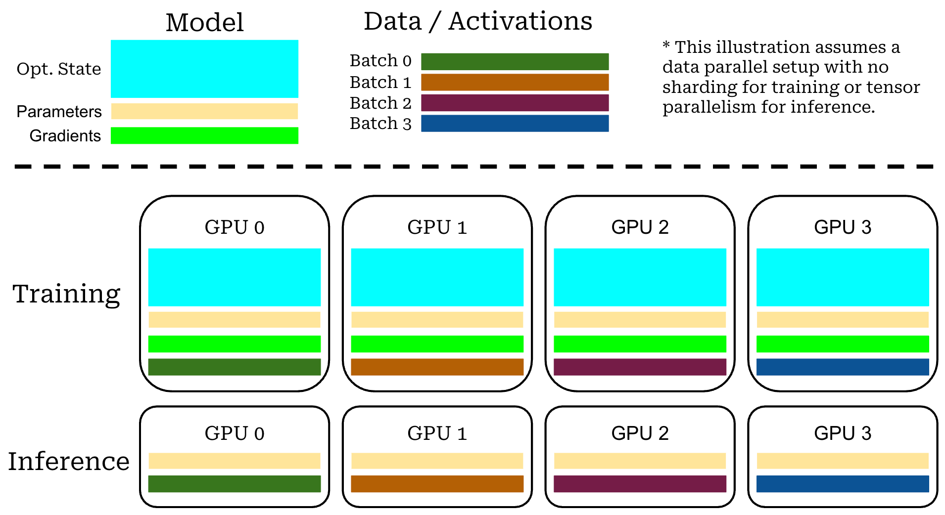
In contrast, training a model in half precision usually requires ~16GB of memory per 1B model parameters, which varies depending on the details of the training setup⁹. Similarly to inference, we load the model weights into GPU memory for training, but we must also store other training-related data (e.g., optimizer states and gradients). We also need enough GPU memory to store model activations during training, so memory consumption still increases with context length.

“As LMs are scaled up, computing gradients for backpropagation requires a prohibitive amount of memory—in our test, up to 12× the memory required for inference—because it needs to cache activations during the forward pass, gradients during the backward pass, and, in the case of Adam, store gradient history.” - source

With this in mind, the fact that GRPO does not use a critic not only saves on compute costs relative to PPO, but it drastically reduces memory consumption—we are now training a single model instead of two models. Eliminating a trainable model has a much larger impact on memory consumption compared to removing a model that is only used for inference (e.g., the reward model).

GRPO & reward models. GRPO became popular primarily in the context of LRM training with RLVR. For this reason, GRPO is mostly used in verifiable reward settings without a neural reward model. A common misconception about GRPO is that it eliminates the need for a reward model, but GRPO can be used with or without a reward model. In fact, the original GRPO paper used a reward model instead of verifiable rewards [1]! Removing the reward model is a benefit of verifiable rewards, not an intrinsic benefit of GRPO itself—the primary advantage of GRPO is the elimination of the critic.

Implementing GRPO

To make this discussion more concrete, let’s implement the GRPO loss function in PyTorch pseudocode. This implementation is adapted from the RLHF book¹⁰, which has a fantastic explanation of GRPO and other policy gradient algorithms.

In the code below, B is our batch size, G is the group size, and L is the context length or number of tokens in each completion. We present two options for approximating KL divergence, including a simple KL estimate (kl_div) that is commonly used for LLMs and a slightly more complex variant (kl_div_alt) that matches the approximation used in the original GRPO paper [1]. More details on why this particular KL divergence estimate is used will be provided later on.

import torch
import torch.nn.functional as F

# constants
kl_beta = 0.1
eps = 0.2

# sample G completions for B prompts
# compute outcome reward for each completion
with torch.no_grad():
    completions = LLM.generate(prompts)  # (B*G, L)
    rewards = RM(completions)  # (B*G)

# create a padding mask from lengths of completions in batch
completion_mask = <... mask out padding tokens ...>

# get policy logprobs for each action
llm_out = LLM(completions)
per_token_logps = F.log_softmax(llm_out, dim=-1)  # (B*G, L)

# get reference logprobs for each action
ref_out = REF(completions)
ref_per_token_logps = F.log_softmax(ref_out, dim=-1)  # (B*G, L)

# compute KL divergence between policy and reference policy
kl_div = per_token_logps - ref_per_token_logps

# alternative KL divergence used by DeepSeekMath [1]
kl_div_alt = (
    torch.exp(ref_per_token_logps - per_token_logps)
    - (ref_per_token_logps - per_token_logps)
    - 1
)

# compute mean and std of grouped rewards
reward_mean = rewards.view(-1, G).mean(dim=1)  # (B,)
reward_std = rewards.view(-1, G).std(dim=1)  # (B,)

# compute advantage for GRPO
advantage = (rewards.view(-1, G) - reward_mean)
advantage /= (reward_std + 1e-8)  # (B, G)
advantage = advantage.view(-1, 1)  # (B*G, 1)

# compute the policy ratio
policy_ratio = torch.exp(
    per_token_logps - old_per_token_logps,
)  # (B*G, L)
clip_policy_ratio = torch.clamp(
    policy_ratio,
    min=1.0 - eps,
    max=1.0 + eps,
)

# compute clipped loss
loss = torch.min(
    advantage * policy_ratio,
    advantage * clip_policy_ratio,
)  # (B*G, L)

# kl divergence added as penalty term to loss
loss = -loss + kl_beta * kl_div

# aggregate the loss across tokens (many options exist here)
loss = ((loss * completion_mask).sum(axis=-1) /
        completion_mask.sum(axis=-1)).mean()

# perform policy gradient update
optimizer.zero_grad()
loss.backward()
optimizer.step()

The implementation above relies upon old_per_token_logps to compute the policy ratio. The old policy refers to the initial policy parameters prior to any policy updates being performed for a batch of data. Before the first update for a batch, we must store these log probabilities so that they can be used for several subsequent policy updates over the same batch. The code above only outlines a single policy update, but if this were our first update over a batch of data we could simply set old_per_token_logps = per_token_logps.detach(). Then, we could re-run this code—excluding the part that samples new completions and computes their rewards—to perform several policy updates over the batch.

Key Publications with GRPO

We now understand the key ideas underlying GRPO, which are relatively simple compared to optimizers like PPO. Next, we will build upon this understanding by outlining a few key papers that demonstrate the practical application of GRPO. Specifically, we will review DeepSeekMath [1] and DeepSeek-R1 [8]. The former paper proposed the GRPO algorithm in the context of training specialized LLMs for solving math problems. This work was later extended by DeepSeek-R1, which used GRPO to train a state-of-the-art open LRM using RLVR. As we will see, this was the first open model to nearly match the performance of closed LRMs like OpenAI’s o1 [9], which led to a subsequent explosion of open LRM releases.

DeepSeekMath: Pushing the Limits of Mathematical Reasoning in Open Language Models [1]

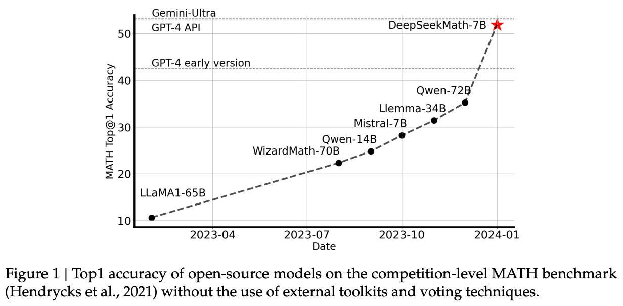
GRPO was proposed with the release of DeepSeekMath [1], a small and open language model for mathematical reasoning. DeepSeekMath uses a combination of i) continued pretraining on a high-quality, math-focused corpus and ii) further training with RL to surpass the performance of similar open-source LLMs—and nearly match the performance of top proprietary models like GPT-4; see below.

(from [1])

Despite its far-reaching impact, GRPO was first proposed in [1] specifically for training domain-specific LLMs. Authors cite simplicity and memory efficiency as key benefits of GRPO relative to PPO. Additionally, we see in [1] that further RL finetuning via GRPO boosts the mathematical reasoning capabilities of even strong models that have already undergone extensive instruction tuning.

“Our research provides compelling evidence that the publicly accessible Common Crawl data contains valuable information for mathematical purposes…. We successfully construct the DeepSeekMath Corpus, a high-quality dataset of 120B tokens from web pages filtered for mathematical content.” - from [1]

The DeepSeekMath Corpus is a high-quality corpus of 120B math-focused tokens—mined from CommonCrawl—used for continued pretraining of DeepSeekMath models. The impressive performance of DeepSeekMath is partially attributed to the “meticulously engineered data selection pipeline” that produces this data. The high-level structure of this data selection pipeline is depicted below.

(from [1])

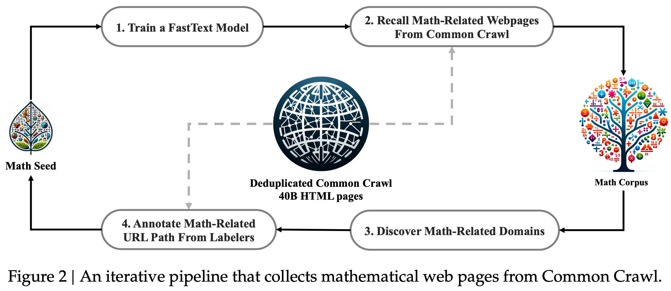
The DeepSeekMath corpus is created iteratively. During the first iteration of data selection, we train a fastText model to identify high-quality math content by using OpenWebMath [2] as a seed corpus. In other words, the OpenWebMath data is used as positive examples of high-quality math content, and we sample 500,000 data points from CommonCrawl to serve as negative examples (i.e., data that are not math-focused). The fastText model is then trained over this data to classify high-quality math content. After deduplicating the web pages in CommonCrawl, we have ~40B web pages that are then ranked by the output of the fastText model—the 40B top-scoring tokens are retained for further refinement.

We further refine this fastText classifier by grouping CommonCrawl into domains with the same base URL. A domain is considered to be “math-related” if more than 10% of the pages in this domain have been identified as math-related by the fastText model. Human annotators manually annotate the URLs in these math-related domains, allowing more math-focused examples to be identified for retraining the fastText model. This process is repeated three times, yielding a total of 120B math-focused tokens. Data collection ends after the fourth iteration because authors found that 98% of the identified data was already collected.

(from [1])

Is the data good? To validate the DeepSeekMath corpus’ quality, pretraining experiments are performed over several different datasets. Models trained on the DeepSeekMath corpus clearly lead on all downstream benchmarks. As shown above, the performance of these models has a steeper learning curve, indicating that the average quality of the DeepSeekMath corpus is higher relative to other math-focused corpora. Additionally, this new corpus is multilingual—primarily English and Chinese—and nearly an order of magnitude larger than alternatives.

DeepSeekMath-Base is the initial base model trained in [1] for mathematical reasoning. It is initialized with the weights of a code model—DeepSeek-Coder-7B-Base-v1.5 in particular—and undergoes continued pretraining on 500B tokens from the DeepSeekMath corpus (and other sources like arXiv papers, Github code, and general language data). DeepSeekMath-7B-Base outperforms other open-source base models on mathematical reasoning—both with and without tool use—and formal theorem proving tasks. Going further, we see in [1] that DeepSeekMath-7B-Base also retains key capabilities in other domains. For example, its performance on coding and general language / reasoning tasks is still strong.

“DeepSeekMath-Base 7B exhibits significant enhancements in performance on MMLU and BBH… illustrating the positive impact of math training on language understanding and reasoning… by including code tokens for continual training, DeepSeekMath-Base 7B effectively maintains the performance of DeepSeek-Coder-Base-v1.5 on the two coding benchmarks.” - from [1]

(from [3, 4, 5])

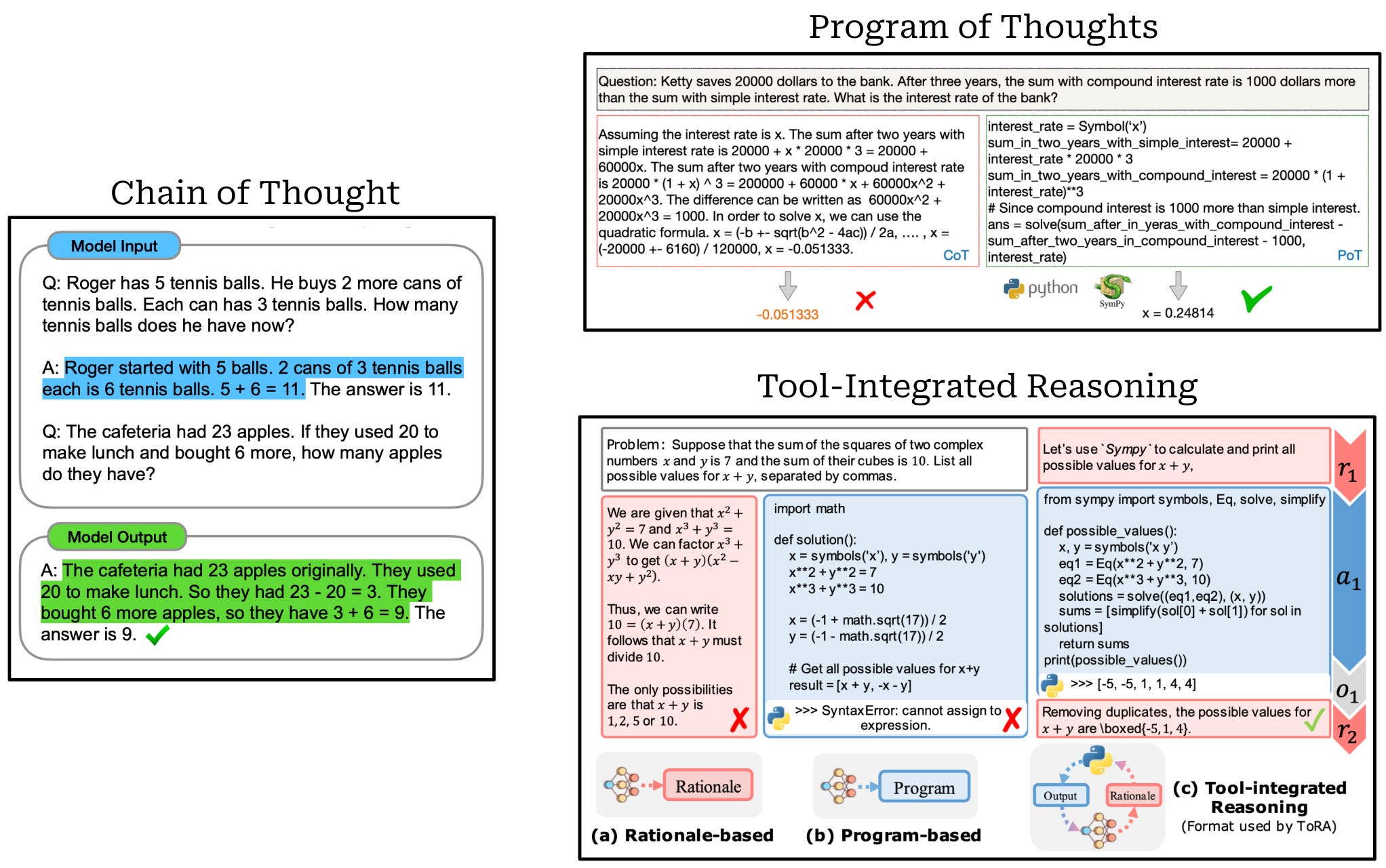
Instruction tuning. After continued pretraining, DeepSeekMath-Base undergoes an instruction tuning phase in which the model is trained with supervised finetuning (SFT) over a curated dataset for mathematical reasoning. Authors collect a set of math problems in both English and Chinese that span diverse fields and levels of complexity. Solutions to these problems are created using three different formats (depicted above):

• Chain of Thought [3]: prompts the model to output intermediate reasoning steps prior to its final answer.

• Program of Thoughts [4]: separates reasoning from computation by prompting the model to output its reasoning steps as a structured program that is then solved by an external code interpreter.

• Tool-Integrated Reasoning [5]: teaches the model to perform complex mathematical reasoning via a trajectory of interleaved natural language reasoning and tool usage (e.g., computation libraries or symbolic solvers).

The final instruction tuning dataset contains a total of 776K examples and is used to train DeepSeekMath-7B-Instruct, starting from DeepSeekMath-7B-Base. As shown below, the instruction tuned model outperforms all other open-source models—even those that are much larger—on chain of thought and tool-integrated reasoning tasks. The model can perform relatively well with or without tools. DeepSeekMath-7B-Instruct also rivals the performance of proprietary models (e.g., Gemini Pro) in some cases but tends to lag behind top-performing models (e.g., Gemini Ultra and GPT-4), especially in the tool-integrated domain.

(from [1])

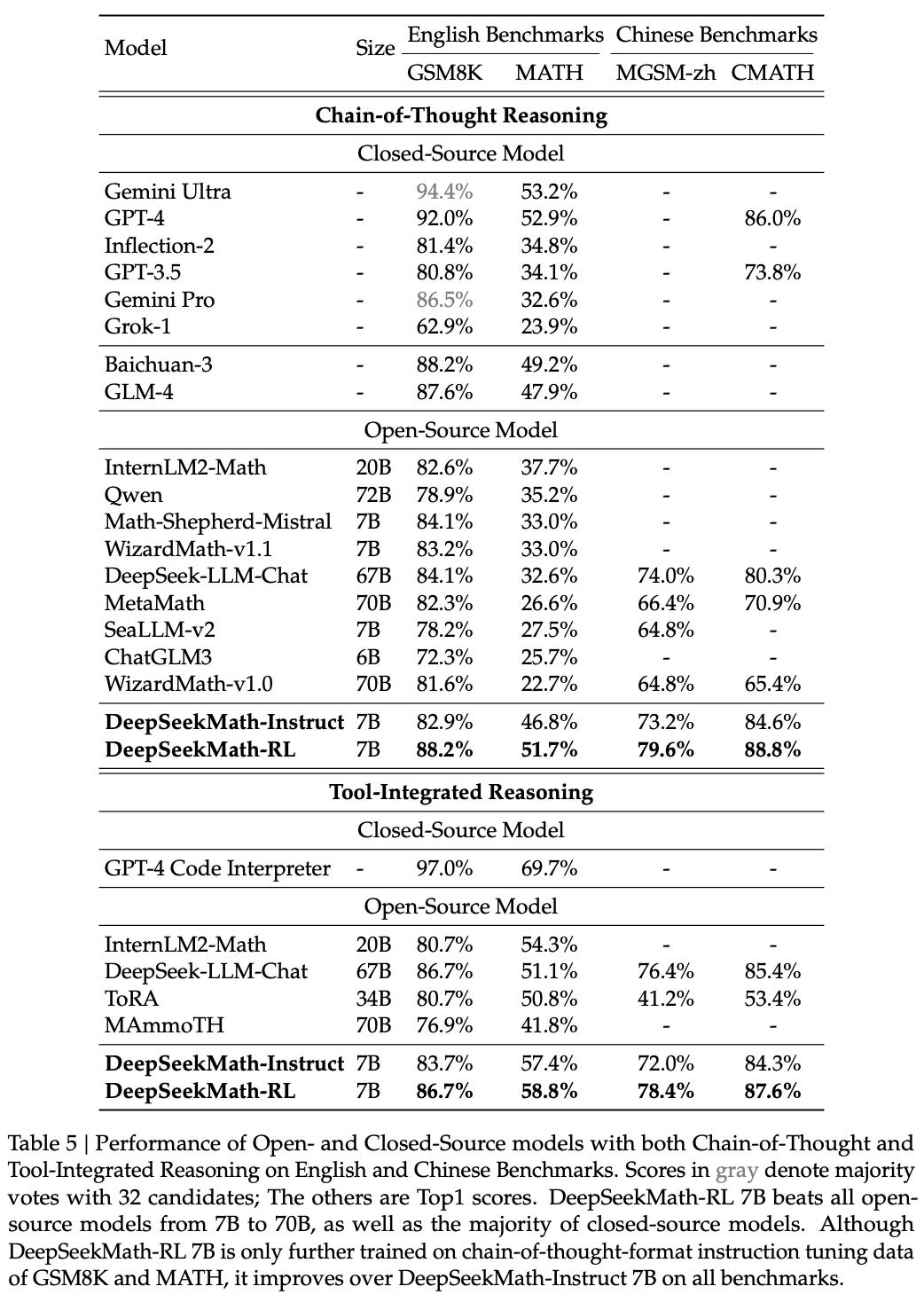
RL training with GRPO. The above table also presents the performance of DeepSeekMath-RL, which undergoes one final RL training phase using GRPO as the underlying optimizer. In fact, GRPO was initially proposed in [1], where authors cite the practicality of GRPO—specifically its memory efficiency, compute efficiency, and simplicity relative to PPO—as key design criteria. Although GRPO is usually used in tandem with verifiable rewards, authors in [1] score completions using a reward model. Additionally, an outcome reward setting is used, meaning that rewards are assigned at the end of a full completion.

“The group relative way that GRPO… calculates the advantages aligns well with the comparative nature of rewards models, as reward models are typically trained on datasets of comparisons between outputs on the same question.” - from [1]

More GRPO details. DeepSeekMath-7B-Instruct is further trained using GRPO over a subset of data from the instruction tuning set—some subsets of this data are purposely left out to test generalization capabilities. During training, the objective is regularized via an added KL divergence penalty between the current policy and the SFT model (i.e., DeepSeekMath-7B-Instruct). Interestingly, authors in [1] adopt a modified estimator of the KL divergence, as shown below.

Different techniques for approximating the KL divergence

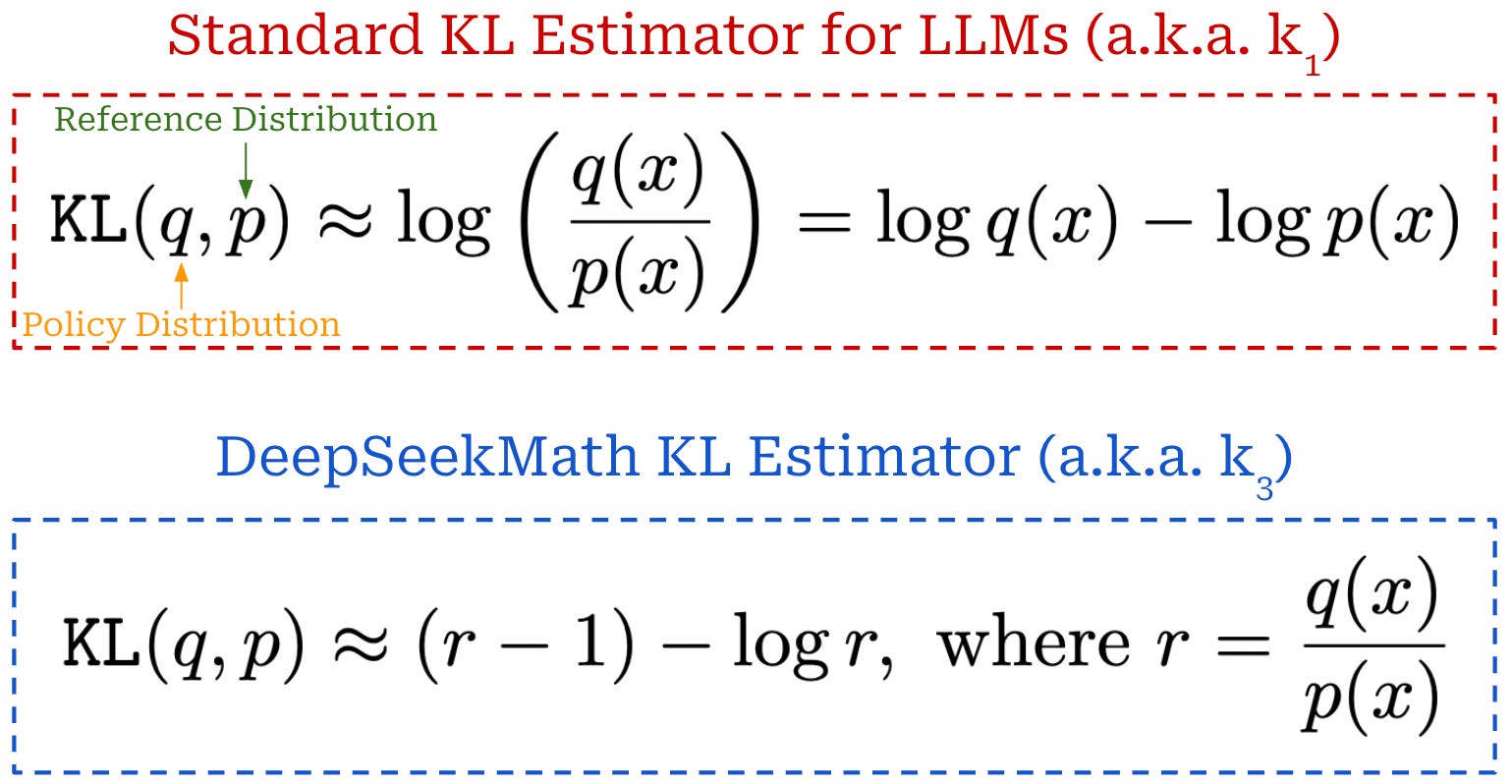
Both of these expressions are valid estimators for the KL divergence; see [7] for details. The estimator for KL divergence that is typically used when training LLMs (top of the figure above) is unbiased but has high-variance. In fact, this estimator can oftentimes be negative in value, whereas the KL divergence is a non-negative metric. In contrast, the estimator used in [1] (bottom of the figure above) is both unbiased and has lower variance—it is guaranteed to be positive—which makes it a desirable estimator for the KL divergence. Due to its use in DeepSeekMath, this estimator has also been adopted in public implementations of GRPO (e.g., this estimator is used in the TRL GRPO trainer).

Training DeepSeekMath-7B-Instruct with GRPO yields the DeepSeekMath-7B-RL model. During GRPO training, we only perform a single policy update for each batch of data. On the other hand, it is common in PPO to perform 2-4 policy updates over the same batch of data [6]. Additionally, GRPO training uses batch sizes that are quite large—a total batch size of 1,024 with 16 prompts and a group size of 64 completions. Large batch sizes are characteristic of GRPO and tend to be a practical necessity for the training process to be stable. As mentioned previously, many samples per prompt are needed because we estimate the advantage purely based on other rewards that are observed within a group.

Impact of RL. After further RL training, DeepSeekMath-7B-RL is found to outperform all open-source models and the majority of proprietary models. Interestingly, the RL-trained model also outperforms DeepSeekMath-Instruct across all benchmarks, despite the constrained scope of its training data—only a small subset of the instruction tuning data (i.e., 144K of 776K total examples) is used during RL. This finding suggests that RL training generalizes well and tends to enhance both in-domain and out-of-domain performance.

“Does code training improve reasoning abilities? We believe it does, at least for mathematical reasoning.” - from [1]

Code, math and beyond. One interesting aspect of the analysis in [1] is the focus upon understanding the interplay between coding and math. As shown in the table below, two training strategies are tested:

• A two-stage pipeline that first trains on either code data or general data, then on math data.

• A one-stage pipeline that (optionally) mixes code data into the math dataset.

In the two-stage pipeline, we see that training the model on coding data—as opposed to general data—prior to training on math data benefits the model’s downstream performance on math benchmarks; see below. This insight motivates initializing DeepSeekMath with the weights of a coding model.

(from [1])

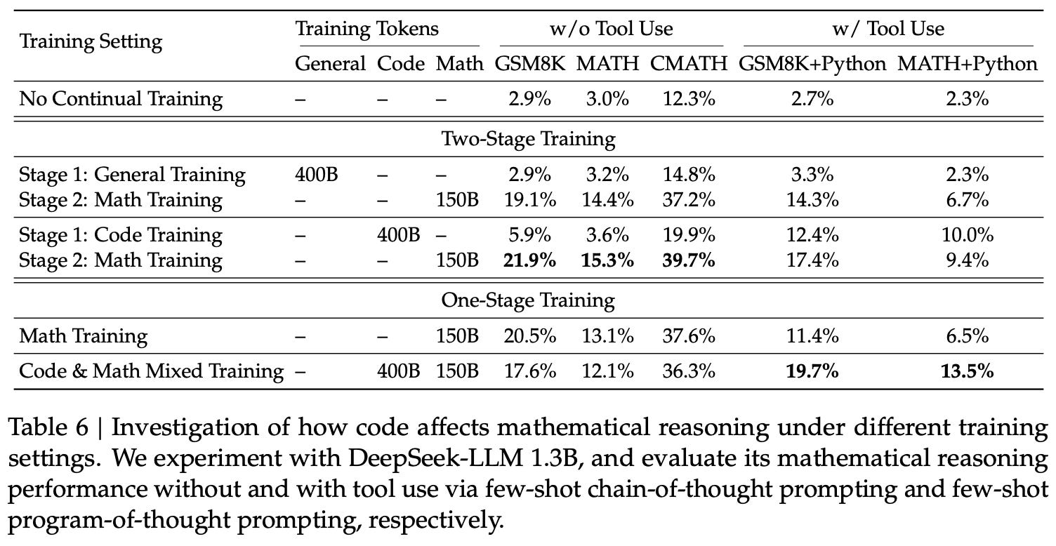
In the one-stage pipeline, the impact of including code data is mixed. Including code in the data mixture helps to avoid catastrophic forgetting and retain coding abilities. However, this data mixture actually degrades performance on certain math benchmarks—particularly those that do not permit tool use—compared to just training on math data. However, this negative result may be due to issues in the data mixture. Namely, the one-stage pipeline uses 150B math tokens and 400B code tokens, which can cause coding capabilities to be prioritized over math.

“We observe the math training also improves model capability on MMLU and BBH benchmarks, indicating it does not only enhance the model’s mathematical abilities but also amplifies general reasoning capabilities.” - from [1]

Beyond studying the interplay between code and math, authors in [1] note that math-focused training tends to improve general model capabilities as well. For example, we see that DeepSeekMath models also have improved performance on general benchmarks like MMLU and BBH, as explained in the quote above.

DeepSeek-R1: Incentivizing Reasoning Capability in LLMs via Reinforcement Learning [8]

(from [8])

Although GRPO was proposed in [1], the algorithm was more widely popularized by its use in training DeepSeek-R1 [8]. During the early days of LRMs, nearly all high-quality reasoning models—such as OpenAI’s o-series models [9]—were closed-source¹¹. For this reason, there was a lot of speculation outside of top labs about how these models actually worked. DeepSeek-R1 [8] was the first open LRM to reach o1-level performance in a transparent way. As detailed in the report, this model is finetuned from DeepSeek-V3 [10]—a 671 billion parameter Mixture-of-Experts (MoE) model—using RLVR. The RL training process uses GRPO and is primarily focused on verifiable domains like math and coding.

(from [9])

Prior to the popularization of LRMs, the scale of RL training performed with LLMs was (relatively) small—post-training was a fraction¹² of total LLM training cost. However, a new kind of scaling law emerged with LRMs [8, 9]; see above. Model performance was shown to smoothly improve with respect to:

1. The amount of compute spent on RL training.

2. The amount of inference-time compute (e.g., by generating multiple outputs or a single output with a longer rationale).

For this reason, the ratio of LLM training cost spent on post-training—and RL in particular—has rapidly increased. In [8], we see exactly this, where DeepSeek-R1 undergoes extensive RL training with GRPO to improve its reasoning abilities.

DeepSeek-R1-Zero is the first model proposed in [8]. This model is initialized with the weights of DeepSeek-V3 [10] and post-trained with large-scale RL. Unlike a standard post-training procedure, no SFT training is used for training R1-Zero—the model is trained purely with GRPO. Interestingly, we see in [8] that R1-Zero naturally learns through RL to leverage its reasoning trajectory to solve complex problems. This was the first open research effort to show that reasoning abilities could be developed in an LLM without supervised training.

“DeepSeek-R1-Zero, a model trained via large-scale reinforcement learning (RL) without supervised fine-tuning (SFT) as a preliminary step, demonstrates remarkable reasoning capabilities. Through RL, DeepSeek-R1-Zero naturally emerges with numerous powerful and intriguing reasoning behaviors.” - from [1]

This model was created by the same authors of DeepSeekMath [1], so R1-Zero also uses GRPO for RL training. Authors cite familiar reasons for this choice:

• Reducing the computational cost of RL training.

• Memory savings from eliminating the critic model.

Verifiable rewards. Authors in [8] choose to avoid using neural reward models when training R1-Zero due to issues with reward hacking in larger-scale RL training runs. Put simply, if we train the LLM for long enough, it will eventually figure out an exploit for the reward model. To solve this issue, R1-Zero is trained using RLVR—using only verifiable reward signals makes the RL training process harder to game. More specifically, two types of rewards are used:

1. Accuracy reward: evaluates whether the model’s response is correct.

2. Format reward: enforces a desired format on the model’s output.

The accuracy reward is computed using task-specific heuristics. For math problems, the model can provide its answer in a specified format, allowing us to verify via basic string matching. Similarly, coding problems can be verified by executing the code produced by the LLM in a sandbox over predefined test cases. In contrast, the format reward simply rewards the model for formatting its output correctly. As shown below, the output format for R1-Zero just uses special tokens to separate the model’s reasoning process from its final output or answer.

(from [8])

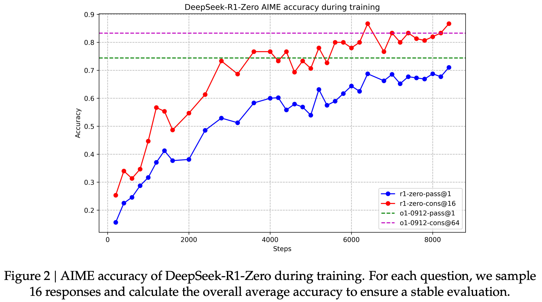
Matching o1. Despite using no SFT, R1-Zero shows clear progress in its reasoning capabilities. The model’s performance on AIME 2024 is plotted below as RL training progresses. Here, we see that performance improves smoothly with the amount of RL training, eventually reaching parity with o1-preview.

(from [8])

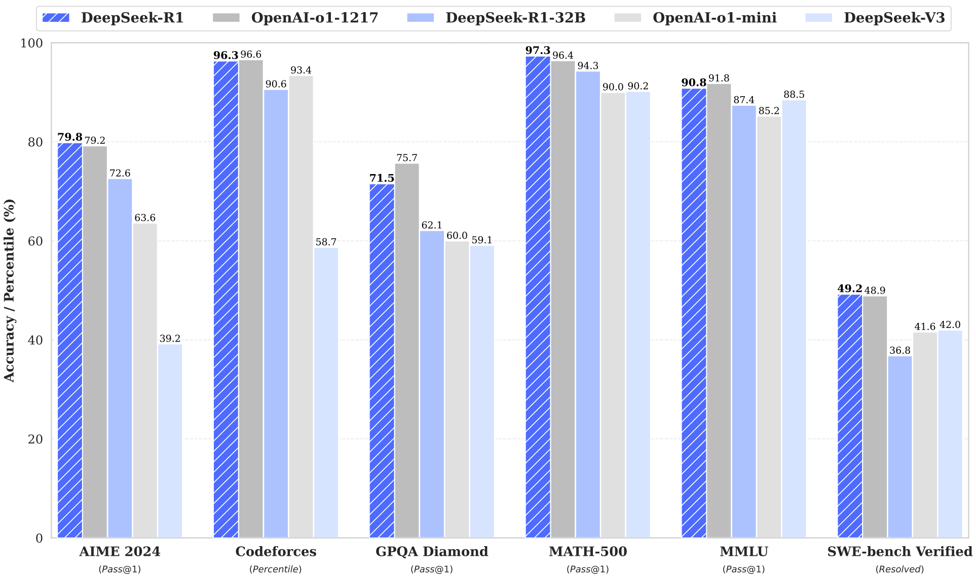
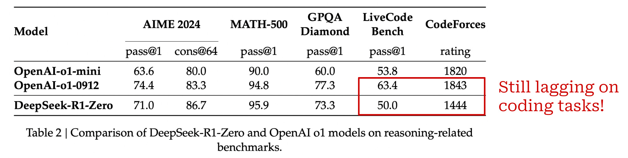
A performance comparison between R1-Zero and o1 models from OpenAI is provided below. R1-Zero matches or exceeds the performance of o1-mini in most cases and performs comparably to o1-preview on several tasks. However, R1-Zero is clearly outperformed by o1 models on coding tasks. As we will see, however, this coding issue was fixed in future iterations of the model.

The beauty of RL. We might begin to wonder how R1-Zero develops such impressive reasoning capabilities during RL training. Luckily, the model’s learning process is observable—we can just monitor the reasoning traces produced by the model over time. By doing this, we see (as shown below) that R1-Zero learns to generate progressively longer chains of thought to improve its reasoning process throughout training. In other words, the model naturally learns that using more inference-time compute is useful for solving difficult reasoning problems.

(from [8])

Additionally, R1-Zero learns to do more than just generate a long chain of thought. Authors in [8] also observe several meaningful behaviors that emerge naturally from RL training. For example, the model develops an ability to reflect upon its own solutions by revisiting and evaluating prior components of its reasoning process. Similarly, the model begins to explicitly test out and explore alternative solutions or approaches while trying to solve a problem.

“The self-evolution of DeepSeek-R1-Zero is a fascinating demonstration of how RL can drive a model to improve its reasoning capabilities autonomously.” - from [8]

Notably, this behavior is not explicitly programmed into the model. Rather, RL allows the model to explore different strategies for arriving at a correct solution. To steer the training process, we reward the model for producing correct answers with proper formatting. From these rewards alone, R1-Zero uses an RL-based “self-evolution” process to naturally learn how to solve reasoning problems. We simply create the correct incentives that facilitate the model’s learning process.

DeepSeek-R1. Despite the impressive reasoning abilities of DeepSeek-R1-Zero, the fact that the model is trained purely with RL—and thus forgoes common best practices for alignment and post-training—causes it to have some bugs. For example, its readability is poor (e.g., no markdown formatting to make its answers easier to read or parse), and it incorrectly mixes languages together. To solve these issues, authors in [8] train the DeepSeek-R1 model, which uses a multi-stage training process to find a balance between standard LLM capabilities and reasoning.

“To prevent the early unstable cold start phase of RL training from the base model, for DeepSeek-R1 we construct and collect a small amount of long CoT data to fine-tune the model as the initial RL actor.” - from [1]

Phase One: SFT Cold Start. Prior to RL training, R1 is trained via SFT over a small dataset of long CoT examples, which is referred to as “cold start” data. This data is collected using a few different approaches:

1. Prompt a model (e.g., DeepSeek-V3) to produce long CoT data, either with few-shot examples or by instructing the model to generate detailed answers with accompanied reflection and verification.

2. Use the R1-Zero model to generate a large number of long CoT outputs, then ask human annotators to post-process and select the model’s best outputs.

Authors in [1] combine these approaches to collect “thousands of cold-start data” on which DeepSeek-V3 is finetuned directly via SFT. Because we are using long CoT data, this is a reasoning-oriented finetuning process. From this cold start data, the model learns a viable (initial) template for solving reasoning problems. The reasoning-oriented SFT data introduces a human prior into training—we have control over the style and pattern of data used in this phase. For example, authors in [1] structure the data to include summaries of each long CoT, which teaches the model to summarize its reasoning process prior to its final answer. We are simply setting a stronger seed from which to start the RL self-evolution process¹³.

Stage Two: Reasoning-Oriented RL. After SFT, we repeat the large-scale RL training process with GRPO (i.e., the same RL training setup used for R1-Zero) to enhance R1’s reasoning capabilities. The only change made for R1 is the addition of a language consistency reward—calculated as the portion of the model’s output written in the desired target language—into RLVR. This language consistency reward is shown in [1] to slightly deteriorate the model’s reasoning capabilities. However, language consistency helps to avoid the language mixing observed in R1-Zero, which makes the model’s output more fluent and readable.

Stage Three: Rejection sampling. After the convergence of reasoning-oriented RL, we use the resulting model to collect a large and diverse SFT dataset. Unlike the initial cold start SFT phase, however, we collect both reasoning-focused and general data, allowing the model to learn from a broader set of domains. The reasoning data for this stage is collected by:

1. Curating a diverse set of reasoning-based prompts.

2. Generating candidate trajectories using the model from after stage two.

3. Performing rejection sampling (i.e., filtering and selecting the top trajectories based on quality and correctness).

Interestingly, the SFT dataset from this stage includes a substantial ratio of non-reasoning data (e.g., writing or translation examples) that is sourced from the post-training dataset for DeepSeek-V3. To match the style of data used for training R1, this data is augmented by adding a CoT—generated by another LLM—to explain the outputs of complex prompts. Simpler prompts are left with no rationale.

“We reuse portions of the SFT dataset of DeepSeek-V3. For certain non-reasoning tasks, we call DeepSeek-V3 to generate a potential chain-of-thought before answering the question by prompting.” - from [1]

Unlike reasoning-oriented data, we cannot use rule-based verification for general-purpose data. Instead, authors in [8] use DeepSeek-V3 as a generative reward model or verifier for this data. After data verification and heuristic filtering (e.g., removing language mixing or long paragraphs), we have a set of 600,000 reasoning examples and 200,000 general-purpose examples, yielding a dataset of 800,000 examples over which we further finetune R1 using SFT.

Stage Four: RLVR & RLHF. The final training stage of R1 aligns the model with human preferences while continuing to hone its reasoning abilities. Similarly to the prior stage, we train the model over a combination of reasoning-based data and general-purpose data reused from the training pipeline of DeepSeek-V3. This stage uses RL with two styles of rewards:

• Rules-based rewards (same as R1-Zero) for reasoning-based problems.

• Neural reward models—trained over human preference pairs, just as in standard RLHF—for general-purpose data.

DeepSeek-R1 is aligned to be more helpful and harmless—two standard alignment criteria for LLMs—on general data. Each criterion is modeled using a separate reward model. For helpfulness, only the final answer (i.e., excluding the long CoT) from the model is passed into the reward model. On the other hand, harmlessness is predicted by passing the entire reasoning trajectory to the reward model. This combination of verifiable and preference-based (neural) rewards allows R1 to be aligned to human preferences while maintaining strong reasoning abilities.

(from [1])

R1 performance. As shown above, R1 matches or surpasses the performance of OpenAI’s o1 model on most reasoning tasks. Unlike R1-Zero, R1 also has strong coding abilities and can handle general-purpose tasks due to its hybrid training pipeline. In general, R1 is a capable model that can handle both traditional and reasoning-oriented tasks. However, we should note that differences exist between LRMs and LLMs—reasoning models are not clearly better in all areas. For example, R1 performs poorly on instruction following benchmarks (e.g., IF-Eval) compared to standard LLMs. However, this trend is likely to be reversed in the future as the balance between standard LLMs and reasoning continues to be refined.

Distilled variants of R1. Given that R1 is a very large model (i.e., 671B parameter MoE), the main R1 model is also distilled to create a series of smaller, dense models. A very simple pipeline is adopted for distillation. Beginning with two base models (i.e., Qwen-2.5 and Llama-3), we simply:

• Generate ~800,000 supervised training examples by sampling completions from the full DeepSeek-R1 model.

• Finetune the base models using SFT over this data.

This is the simplest form of distillation that can be used, which just trains the student on completions from the teacher using SFT. Such an approach is referred to as off-policy distillation [11]. This off-policy distillation procedure works well for the R1 model. In fact, distilling from R1 actually outperforms direct training of smaller models with RL; see below. However, we can usually achieve better performance via logit distillation (i.e., training the student model on the full log probabilities outputted by the teacher for each token) or on-policy distillation.

(from [8])

Conclusion

The advent of large reasoning models has completely transformed LLM research, especially the domain of reinforcement learning. For years, research on RL has centered around complex algorithms like PPO that require substantial domain knowledge and extensive compute resources. As a result, much of the research in this area has been confined to a handful of top research labs. This trend has recently changed, however, as open reasoning models and simpler RL algorithms like GRPO have become increasingly popular. Today, there are more public resources than ever before for doing useful research at the intersection of RL and LLMs. Hopefully, the details outlined in this post will contribute to further democratizing research on this important and rapidly evolving topic.

New to the newsletter?

Hi! I’m Cameron R. Wolfe, Deep Learning Ph.D. and Senior Research Scientist at Netflix. This is the Deep (Learning) Focus newsletter, where I help readers better understand important topics in AI research. The newsletter will always be free and open to read. If you like the newsletter, please subscribe, consider a paid subscription, share it, or follow me on X and LinkedIn!

Bibliography

[1] Shao, Zhihong, et al. “Deepseekmath: Pushing the limits of mathematical reasoning in open language models.” arXiv preprint arXiv:2402.03300 (2024).

[2] Paster, Keiran, et al. “Openwebmath: An open dataset of high-quality mathematical web text.” arXiv preprint arXiv:2310.06786 (2023).

[3] Wei, Jason, et al. “Chain-of-thought prompting elicits reasoning in large language models.” Advances in neural information processing systems 35 (2022): 24824-24837.

[4] Chen, Wenhu, et al. “Program of thoughts prompting: Disentangling computation from reasoning for numerical reasoning tasks.” arXiv preprint arXiv:2211.12588 (2022).

[5] Gou, Zhibin, et al. “Tora: A tool-integrated reasoning agent for mathematical problem solving.” arXiv preprint arXiv:2309.17452 (2023).

[6] Lambert, Nathan. “Reinforcement Learning from Human Feedback.” Online (2025).

https://rlhfbook.com

[7] Schulman, John. “Approximating KL Divergence.” Online (2020). http://joschu.net/blog/kl-approx.html.

[8] Guo, Daya, et al. “Deepseek-r1: Incentivizing reasoning capability in llms via reinforcement learning.” arXiv preprint arXiv:2501.12948 (2025).

[9] OpenAI et al. “Learning to Reason with LLMs.” https://openai.com/index/learning-to-reason-with-llms/ (2024).

[10] Liu, Aixin, et al. “Deepseek-v3 technical report.” arXiv preprint arXiv:2412.19437 (2024).

[11] Lu, Kevin et al. “On-Policy Distillation.” https://thinkingmachines.ai/blog/on-policy-distillation/ (2025).

[12] Schulman, John, et al. “Proximal policy optimization algorithms.” arXiv preprint arXiv:1707.06347 (2017).

[13] Schulman, John, et al. “High-dimensional continuous control using generalized advantage estimation.” arXiv preprint arXiv:1506.02438 (2015).

[14] Team, Kimi, et al. “Kimi k2: Open agentic intelligence.” arXiv preprint arXiv:2507.20534 (2025).

[15] Khatri, Devvrit, et al. “The art of scaling reinforcement learning compute for llms.” arXiv preprint arXiv:2510.13786 (2025).

[16] Ouyang, Long, et al. “Training language models to follow instructions with human feedback.” Advances in neural information processing systems 35 (2022): 27730-27744.

[17] Stiennon, Nisan, et al. “Learning to summarize with human feedback.” Advances in neural information processing systems 33 (2020): 3008-3021.

[18] Bai, Yuntao, et al. “Training a helpful and harmless assistant with reinforcement learning from human feedback.” arXiv preprint arXiv:2204.05862 (2022).

[19] Lambert, Nathan, et al. “Tulu 3: Pushing frontiers in open language model post-training.” arXiv preprint arXiv:2411.15124 (2024).

[20] Bespoke Labs et al. “Scaling up Open Reasoning with OpenThinker-32B.” https://www.bespokelabs.ai/blog/scaling-up-open-reasoning-with-openthinker-32b (2025).

1. In fact, some researchers argue that the distinction between an LLM and an LRM is an unnecessary gray area—they are still the same types of models.

2. Frontier labs have argued that the LRM’s chain of thought is a useful artifact for monitoring the model for harmful behavior. To maintain our ability to monitor, the reasoning process is usually kept “unsafe”—we apply no safety post-training to it to ensure that the model does not learn to omit info from its reasoning process for safety purposes. As a result, the reasoning process is potentially unsafe and will be kept that way for monitoring benefits) and cannot be directly exposed to the end user. Alternatively, top labs could be simply omitting the reasoning trajectory to make distilling from their best reasoning models more difficult.

3. This naming stems from the fact that the surrogate objective is different from the RL training objective. In RL, we aim to maximize cumulative reward. However, directly maximizing this objective can lead to instability. The surrogate is a more stable proxy that can be optimized in place of the true objective.

4. The critic is very similar to a reward model—both models predict rewards. However, the critic predicts reward per-token, while a reward model usually predicts outcome rewards for an entire completion. Additionally, reward models are usually fixed during RL training while the critic is trained alongside the policy itself.

5. The bias comes from relying on an approximate value model for this estimate and only using a small amount of exact reward information r_t.

6. A commonly used setting for λ is ~0.95.

7. The stop gradient is used here because, when using the GRPO loss function, we are computing the gradient of the loss with respect to our policy. Usually, the policy in the denominator of this expression is the old policy. We consider the output of this policy to be a constant when computing the gradient. When performing only a single policy update per batch of data, the old policy is equal to our current policy, but we still consider this denominator term a constant when computing the gradient. This is accomplished via the stop gradient operation.

8. For example, hosting Qwen-3-32B in half precision with its full context length (131K tokens) would increase the memory footprint from ~70GB to ~400GB.

9. This exact number will vary drastically depending on our exact training settings. For example, this calculation assumes that we are using the AdamW optimizer, which maintains three separate optimizer states for every model parameter at full precision (default setting for AdamW parameters and optimizer states). We can reduce memory by using an 8-bit AdamW optimizer. Additionally, we can adopt various sharding (e.g., ZeRO, FSDP, and more) or pipelining strategies if we have multiple GPUs or nodes available for training to reduce per-GPU memory consumption significantly.

10. The implementation also draws upon code from a prior PPO tutorial, as well as the implementation of GRPO in TRL.

11. Some open reasoning models like QwQ preceded the release of DeepSeek-R1.

12. The cost of training an LLM is dominated by pretraining. However, the cost of post-training can still be expensive, especially when human data annotation is considered; see here for more details. Therefore, the ratio of cost spent on post-training varies, but it would generally be <10% of the total LLM training cost.

13. See here for more info on the role of SFT in training reasoning models.