REINFORCE: Easy Online RL for LLMs

How to get the benefits of online RL without the complexity of PPO...

Reinforcement learning (RL) is playing an increasingly important role in research on large language models (LLMs). Initially, RL was used to power LLM alignment via approaches like Reinforcement Learning from Human Feedback (RLHF). More recently, it has become foundational for training powerful large reasoning models (LRMs). When training LLMs with RL, online algorithms such as Proximal Policy Optimization (PPO) are often used by default. However, these algorithms are expensive and complex compared to alternatives like supervised finetuning (SFT) or direct preference optimization (DPO):

• Four different copies of the LLM must be kept in memory.

• The online training process is difficult to orchestrate and can be unstable.

• There are many training hyperparameters that must be tuned properly.

The complexity of PPO arises from the need to stabilize the online training process. This algorithm was developed in an earlier generation of research, which focused on training neural networks from scratch to solve tasks like robotic locomotion and Atari gameplay. The RL setting for LLMs is much different—we are fine-tuning pretrained models that already have a powerful prior.

“PPO has been positioned as the canonical method for RLHF. However, it involves both high computational cost and sensitive hyperparameter tuning. We posit that the motivational principles that led to the development of PPO are less of a practical concern in RLHF and advocate for a less computationally expensive method that preserves and even increases performance.” - from [3]

Many practitioners avoid the use of online RL when training LLMs due to cost and complexity. In this overview, we will learn that online RL does not have to be so difficult! Due to the unique properties of the LLM domain, we can use simpler algorithms—like REINFORCE or REINFORCE leave-one-out (RLOO)—and still achieve performance similar to that of PPO. Therefore, instead of avoiding online RL in favor of simpler RL-free or offline alternatives, we can just use algorithms that provide the benefits of online RL without the unnecessary complexity.

Basics of RL for LLMs

We will begin by covering the basics of reinforcement learning (RL). To start, we will explore the problem setup and terminology commonly used in RL, as well as how these formalisms can be translated to the LLM domain. After covering RL fundamentals and how RL is applied in the context of LLMs, we will spend the majority of this section focusing on policy optimization by deriving the standard policy gradient expression frequently used in RL and outlining concrete implementations for the most basic forms of these training algorithms.

Problem Setup and Terminology for RL

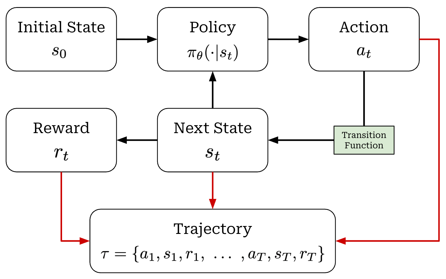
When running RL training, we have an agent that takes actions within some environment; see below.

Basic problem setup for RL

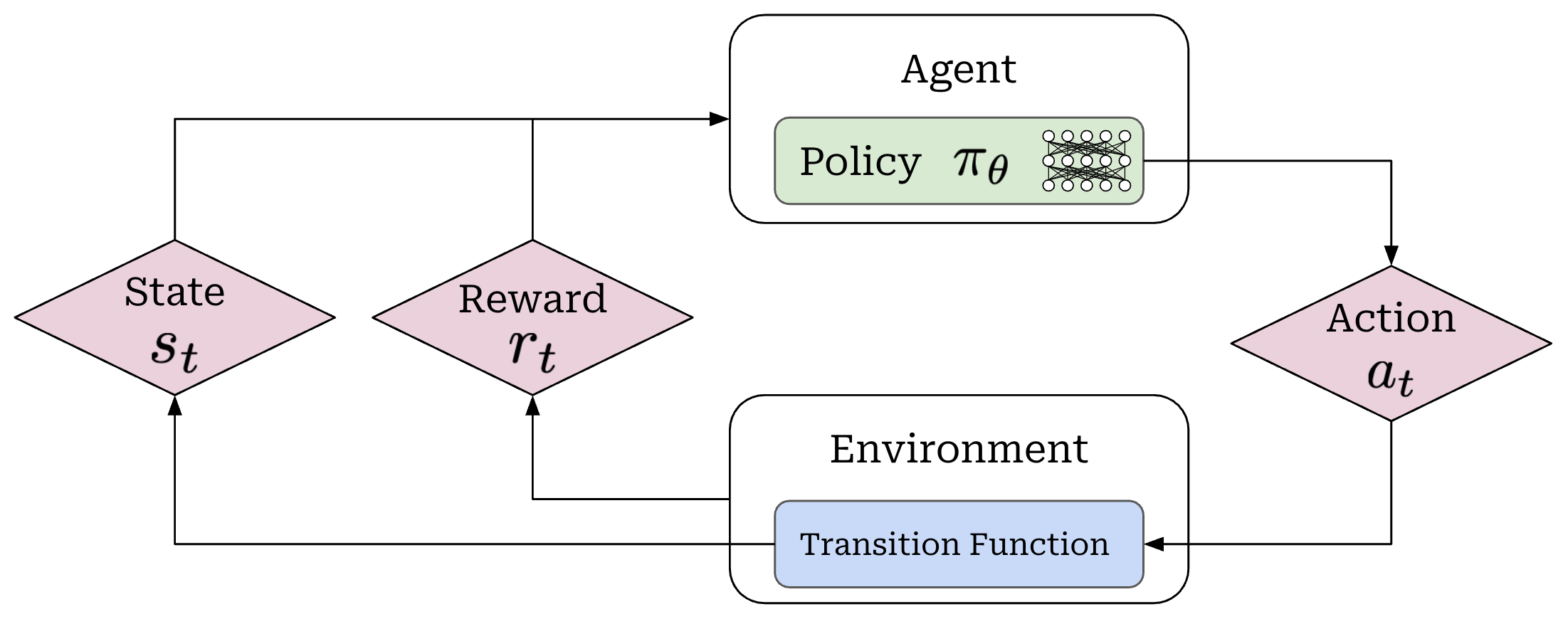
These actions are predicted by a policy—we can think of the policy as the agent’s brain—that is usually parameterized (e.g., the policy is the LLM itself in the context of training LLMs). Our policy can either be deterministic or stochastic, but in this overview we will assume the policy is stochastic¹. We can model the probability of a given action under our policy as π_θ(a_t | s_t).

When the policy outputs an action, the state of the environment will be updated according to a transition function, which is part of the environment. We will denote our transition function as P(s_t+1 | a_t, s_t). However, transition functions are less relevant for LLMs because they are typically a pass-through; i.e., we assume s_t = {x, a_1, a_2, …, a_t}, where x is the prompt.

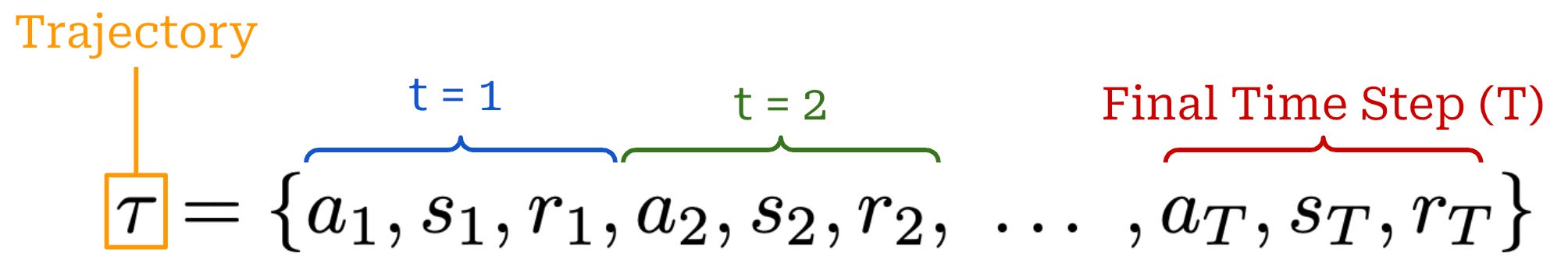
Finally, each state visited by the agent receives a reward from the environment that may be positive, negative, or zero (i.e., no reward). As shown in the prior figure, our agent acts iteratively and each action (a_t), reward (r_t), and state (s_t) are associated with a time step t. Combining these time steps together yields a trajectory; see below. Here, we assume that the agent takes a total of T steps in the environment for this particular trajectory.

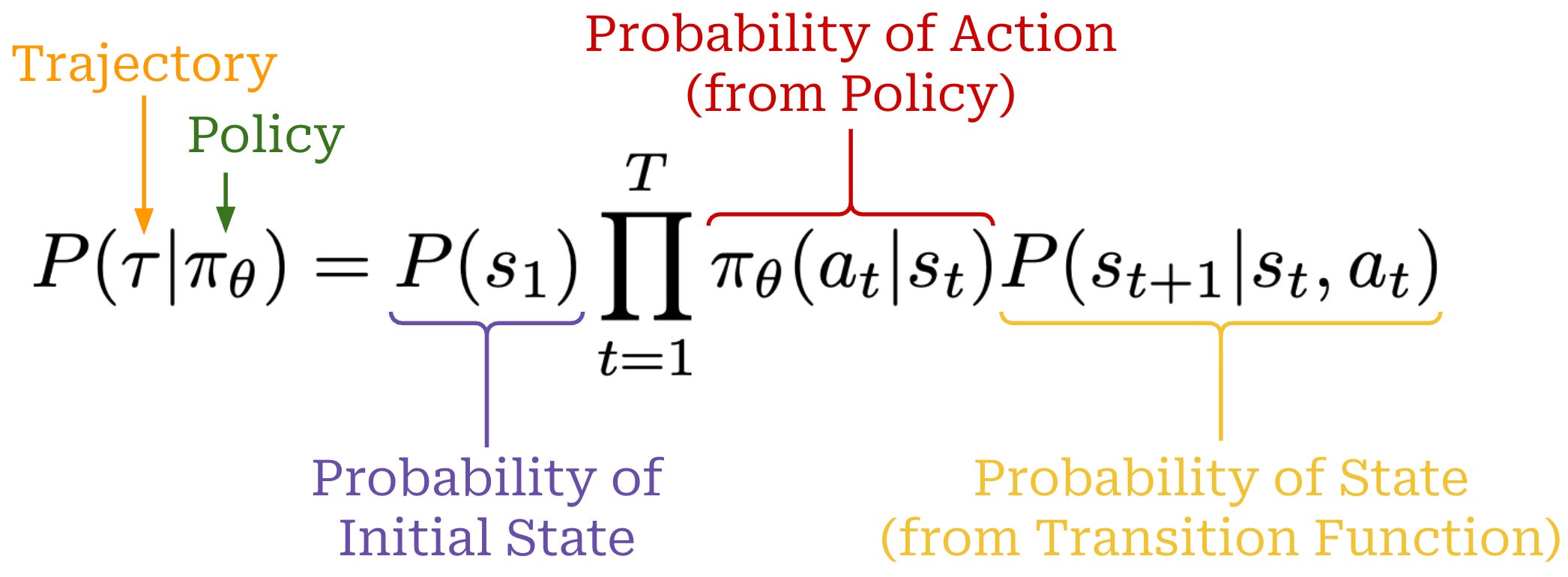
Using the chain rule of probabilities, we can also compute the probability of a full trajectory by combining the probabilities of:

• Each action a_t given by our policy π_θ(a_t | s_t).

• Each state s_t+1 given by the transition function P(s_t+1 | a_t, s_t).

The full expression for the probability of a trajectory is provided below.

Computing the probability of a trajectory

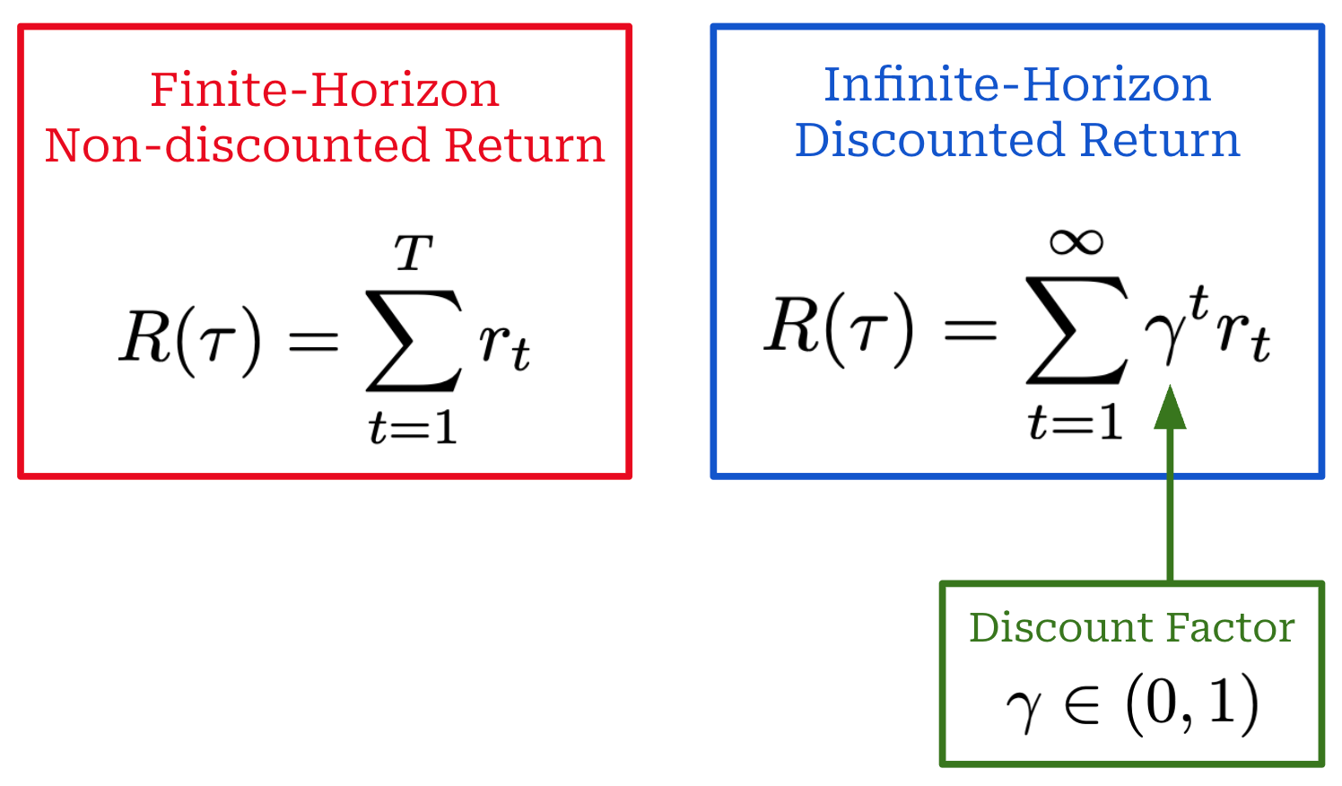
RL objective. When training a model with RL, our goal is to maximize the cumulative reward over the entire trajectory (i.e., the sum of r_t). However, there are a few variations of this objective that commonly appear. Specifically, the reward that we maximize can either be discounted or non-discounted²; see below. By incorporating a discount factor, we reward our policy for achieving rewards sooner rather than later. In other words, money now is better than money later.

Our objective is usually expressed as an expected cumulative reward, where the expectation is taken over the trajectory. Expanding this expectation yields a weighted sum of rewards for each trajectory—the weight is just the trajectory’s probability. We can formulate this in a continuous or discrete manner; see below.

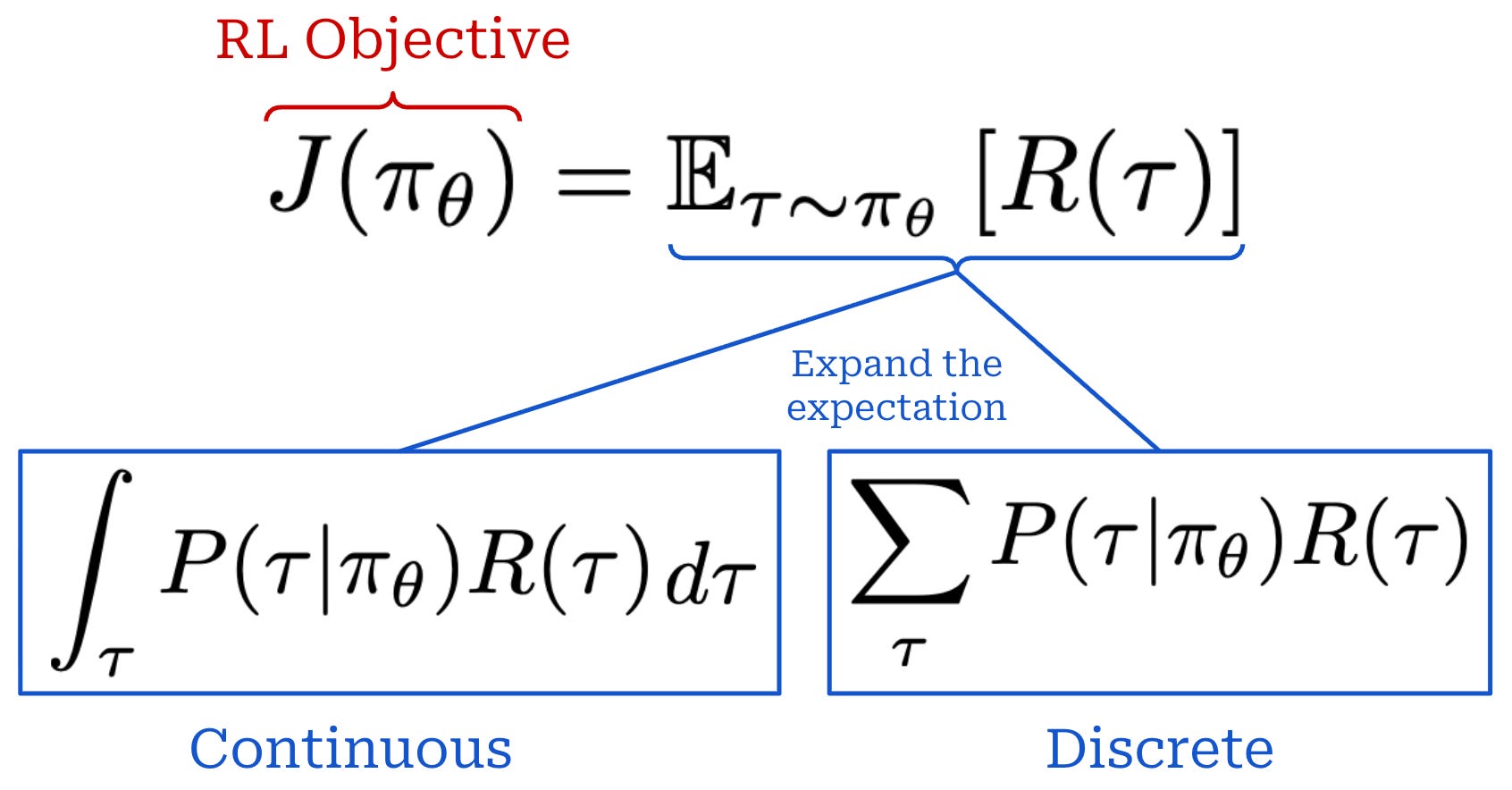
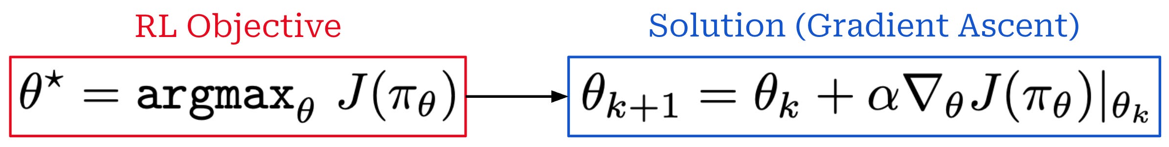
We want to maximize this objective during training, which can be accomplished via gradient ascent³; see below. Given this setup, the lingering question that we have to answer is: How do we compute this gradient? As we will see, much of the research on RL focuses on answering this question, and many techniques exist.

Solving the RL objective with gradient ascent

State, value, and advantage functions. Related to RL objective, we can also define the following set of functions:

• Value Function V(s): the expected cumulative reward when you start in state s and act according to your current policy π_θ.

• Action-Value Function Q(s, a): the expected cumulative reward when you start in state s, take action a, then act according to your policy π_θ.

• Advantage Function A(s, a): the difference between the action-value and value function; i.e., A(s, a) = Q(s, a) - V(s).

Intuitively, the advantage function tells us how useful some action a is by taking the difference between the expected reward after taking action a in state s and the general expected reward from state s. The advantage will be positive if the reward from action a is higher than expected and vice versa. Advantage functions play a huge role in RL research—they are used to compute the gradient for our policy.

“Sometimes in RL, we don’t need to describe how good an action is in an absolute sense, but only how much better it is than others on average. That is to say, we want to know the relative advantage of that action. We make this concept precise with the advantage function.” - Spinning up in Deep RL

Markov Decision Process (MDP) versus Bandit Formulation

RL terminology mapping for LLMs

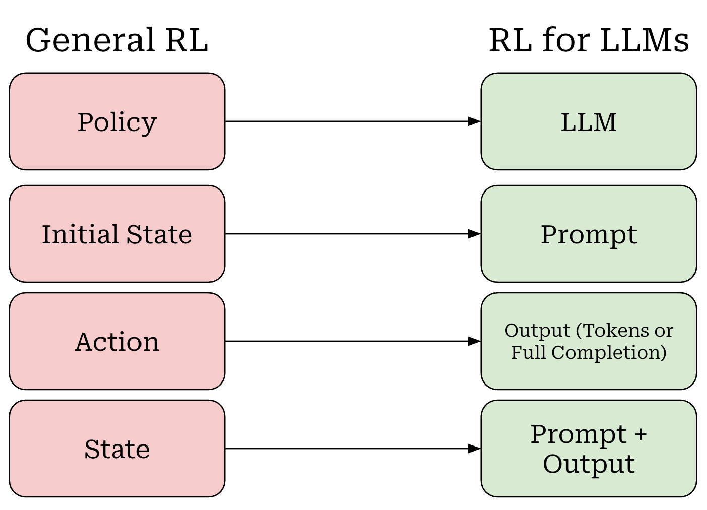
Now that we understand RL basics, we need to map the terminology that we have learned to the setting of LLM training. We can do this as follows (shown above):

• Our policy is the LLM itself.

• Our initial state is the prompt.

• The LLM’s output—either each token or the entire completion—is an action.

• Our state is the combination of our prompt with the LLM’s output.

• The entire completion from the LLM forms a trajectory.

Notably, there is no transition function in this setup because the transition function is completely deterministic. If we start with a prompt x and our LLM predicts tokens t_1 and t_2 given this prompt as input, then our updated state simply becomes s_2 = {x, t_1, t_2}. In other words, our state is just the running completion being generated by the LLM for a given prompt x.

Markov decision process (MDP) formulation. For LLMs, there are two key ways in which RL can be formulated that differ in how they model actions. We should recall that an LLM generates output via next token prediction; i.e., by generating each token in the output completion sequentially. This autoregressive process is depicted below. As we can see, the next token prediction process maps very easily to an RL setup—we can just model each token as an individual action!

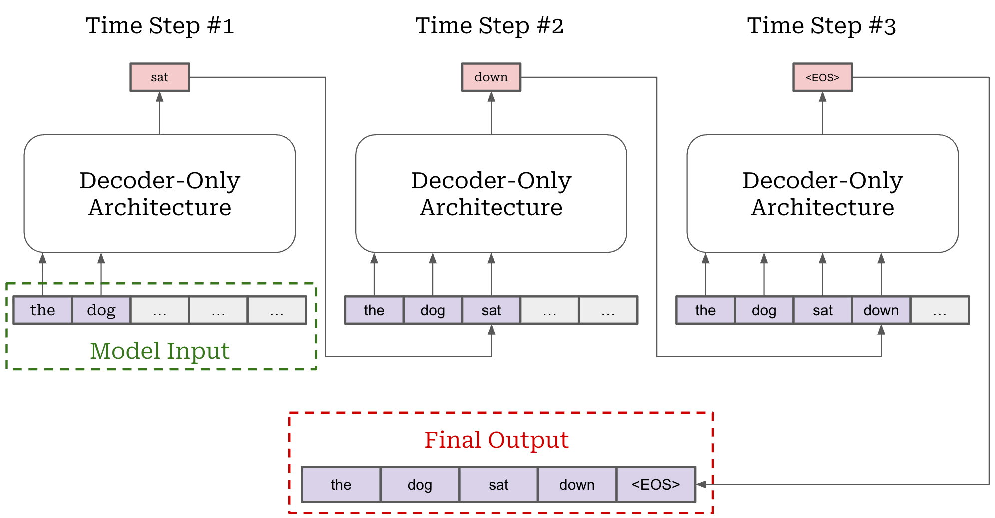
The approach of modeling each token in the LLM’s output as an individual action is called the Markov Decision Process (MDP) formulation. An MDP is simply a probabilistic framework for modeling decision-making that includes states, actions, transition probabilities and rewards—this is exactly the setup we have discussed so far for RL! The MDP formulation used for RL is shown below.

When modeling RL as an MDP for LLMs, our initial state is the prompt and our policy acts by predicting individual tokens. Our LLM forms a stochastic policy that predicts a distribution over tokens. During generation, actions are taken by selecting a token from this distribution—each token is its own action. After a token is predicted, it is added to the current state and used by the LLM to predict the next token—this is just autoregressive next token prediction! Eventually, the LLM predicts a stop token (e.g., <|end_of_text|> or <eos>) to complete the generation process, thus yielding a complete trajectory.

Bandit formulation. In the above depiction of an MDP, we assume that a reward is provided for every time step, but the reward mechanism for an LLM is usually a bit different from this. Most LLMs are trained using outcome supervision⁴, meaning that a reward is only assigned after the model has generated a complete response (i.e., after the <eos> token has been outputted).

Outcome versus process supervision for LLMs

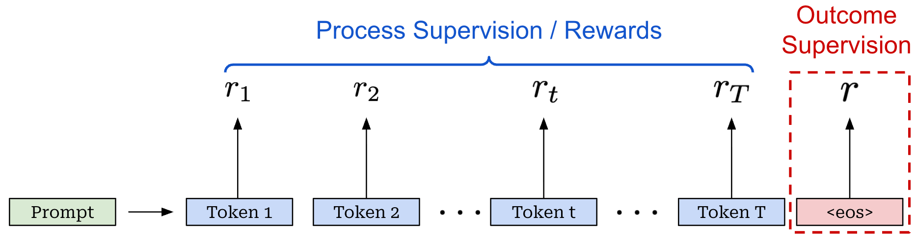
In an outcome supervision setting, we may begin to question the utility of modeling each token as its own action. How will we know whether any single action is helpful or not in this scenario? As an alternative, we could model the entire response as a single action that receives an outcome reward. This is the key idea behind the bandit formulation for RL training with LLMs; see below.

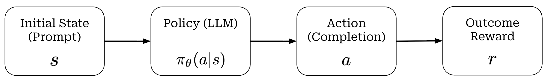
This name comes from the idea of a contextual bandit in probability theory. The bandit setup is simple: our agent chooses an action, receives a reward and the episode ends. Our complete trajectory is a single action and reward! For LLMs, our action is the full completion generated for a prompt, which receives an outcome reward.

Which formulation should we use? In the context of LLMs, we already know how to compute the probability of both individual tokens and the full completion for a prompt. Therefore, we have the ability to model RL using either an MDP or bandit formulation. Given that LLMs usually only receive outcome rewards, however, the bandit formulation—despite being very simple—is quite fitting for LLMs. As we will learn, both REINFORCE and RLOO adopt the bandit formulation, while algorithms like PPO use a per-token MDP formulation. In other words, both RL formulations are viable and used for training LLMs.

RL Training for LLMs

Given the terminology and setup explained so far, we can now discuss how RL is actually used to train LLMs. There are two broad categories of RL training that are commonly used for LLMs today:

• Reinforcement Learning from Human Feedback (RLHF) trains the LLM using RL with rewards derived from a human preference reward model.

• Reinforcement Learning with Verifiable Rewards (RLVR) trains the LLM using RL with rewards derived from rules-based or deterministic verifiers.

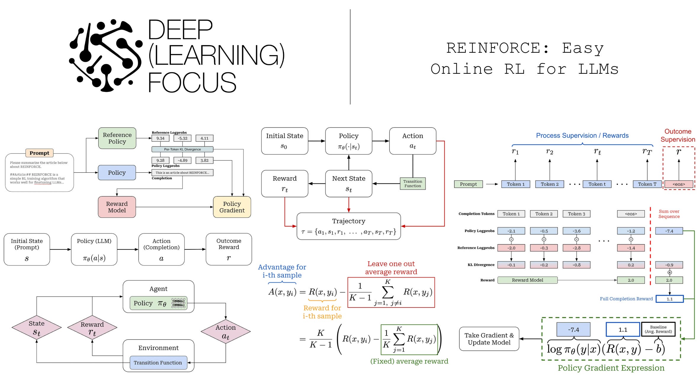
These RL training techniques differ mainly in how they derive the reward for training, but other details of the algorithms are mostly similar. As depicted below, they both operate by generating completions over a set of prompts, computing the reward for these completions, and using the rewards to derive a policy update—or an update to the LLM’s parameters—with an RL optimizer.

Visual depiction of RL for LLMs

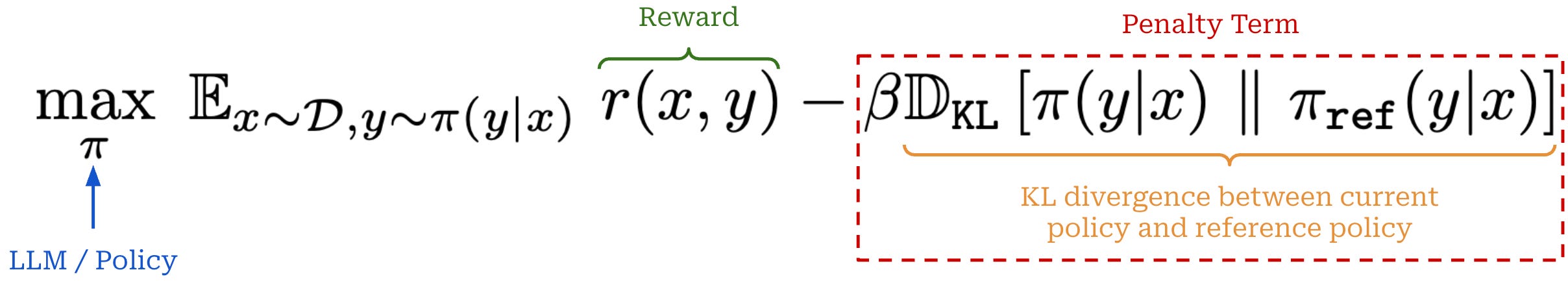
The last step of this process is a gradient ascent step on the RL objective, just as we saw before. However, the actual objective used in RL training goes beyond maximizing cumulative reward. We try to maximize the reward while minimizing KL divergence of our policy with respect to a reference policy—usually an LLM checkpoint from the start of RL training. We want to maximize reward without making our new model significantly different from the reference; see below.

RL training objective with KL divergence

Computing the gradient of this objective with respect to the policy’s parameters is where most of the complexity lies in understanding RL. In the context of LLMs, we use policy gradient algorithms (e.g., PPO, GRPO, and REINFORCE) to compute this gradient. This overview will primarily focus on REINFORCE and its variants, but to learn how these algorithms work we need to first understand the simplest form of a policy gradient—the vanilla policy gradient (VPG).

Deriving the Vanilla Policy Gradient (VPG)

We will cover the full derivation of the vanilla policy gradient (VPG) here for completeness. However, there are many existing overviews that explain VPG very well. A few great resources for further learning are as follows:

• Intro to Policy Optimization from OpenAI [link]

• RLHF Book from Nathan Lambert [link]

• Policy Optimization Algorithms from Lilian Weng [link]

Additionally, the prior breakdown of VPG and policy optimization from this newsletter is linked below for easy reference. Our discussion in this section will largely be sampled from this more detailed exposition of policy gradients.

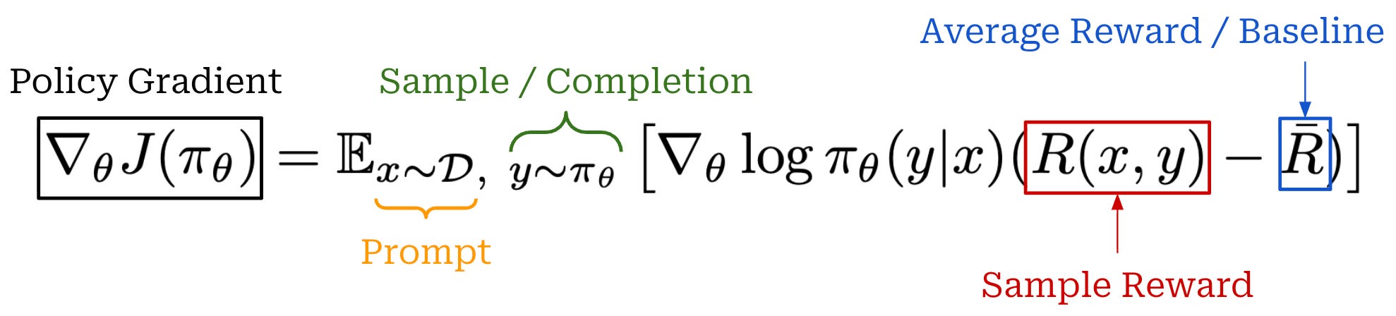
A basic policy gradient. Our goal in policy optimization is to compute the policy gradient, or the gradient of our RL objective—here we will assume our objective is cumulative reward—with respect to the parameters of our policy. As a first step in computing the policy gradient, we can perform the derivation shown below.

(source)

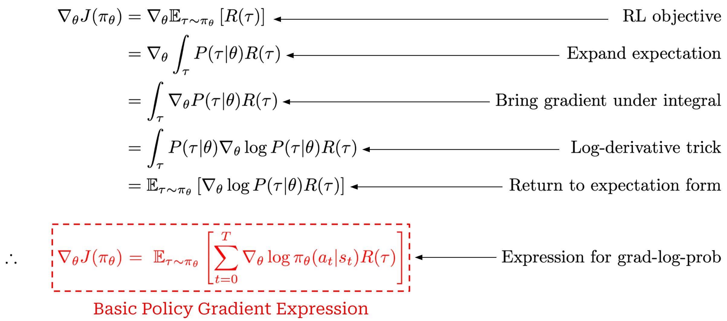
This derivation starts with the gradient of our RL training objective (cumulative reward) and ends with a basic expression for the policy gradient. To arrive at the policy gradient, we use mostly simple steps like i) the definition of an expectation over a continuous random variable and ii) the log-derivative trick.

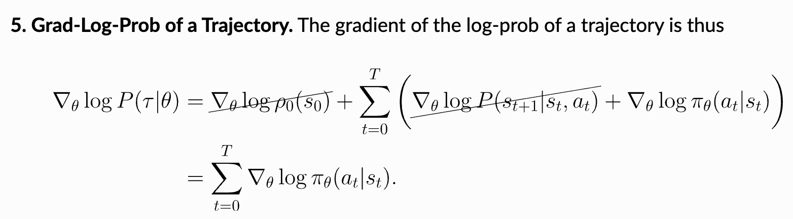
The most complicated step of this derivation is the final step, which transforms the gradient of the log probability of a trajectory into a sum over the gradients of log probabilities of actions. This step uses our prior expression for the probability of a trajectory, converts the product into a sum (i.e., because we are working with log probabilities), and observes that the gradients of the initial state probability and transition function with respect to the policy parameters are always zero because neither of these components depend on the policy; see below.

(source)

Implementing a basic policy gradient. The basic policy gradient expression that we derived above is actually pretty easy to compute. Specifically, this expression contains two key quantities that we already know how to compute:

• The reward comes directly from a verifier or reward model.

• Log probabilities of actions can be computed with our LLM (i.e., these are just the token probabilities from the LLM’s output).

To make the process of computing the basic policy gradient more concrete, a step-by-step implementation in PyTorch pseudocode has been provided below.

The core intuition behind the structure of this basic policy gradient is that we are increasing the probability of actions from trajectories with high rewards.

“Taking a step with this gradient pushes up the log-probabilities of each action in proportion to R(𝜏), the sum of all rewards ever obtained.” - Spinning up in Deep RL

This form of the policy gradient is simple, but it still appears in practice! For example, Cursor uses this exact expression in their recent blog on online RL. However, the expression in their blog assumes a bandit formulation, which causes the sum in the expression to be removed (i.e., because there is only one action).

(source)

Reducing variance. Our current policy gradient expression is simple, but it suffers from a few notable issues:

• The gradients can have high variance.

• There is no protection against large, unstable policy updates.

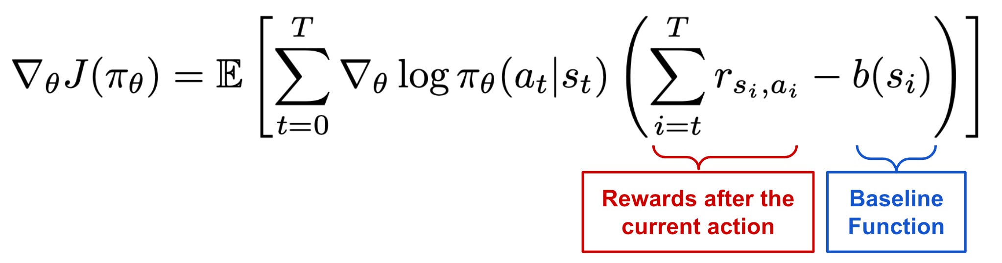
Most subsequent policy gradient algorithms aim to solve these problems by reducing variance of the policy gradient and enforcing a trust region on policy updates—or, in other words, restricting how much we can change the model in a single update. To do this, we usually replace the reward term in our policy gradient with a slightly different term; see below for some of the common options.

(from [4])

As we can see, this expression is nearly identical to what we saw before. The only difference is that we have switched R(𝜏) with the generic Ψ_t term, which can be set equal to a couple of different things. For example, we can:

• Set Ψ_t = R(𝜏) to recover our basic policy gradient expression.

• Set Ψ_t equal to rewards received after time t (i.e., the reward-to-go policy gradient) to avoid crediting actions with rewards that came before them.

• Set Ψ_t to a baselined version of the reward.

• Set Ψ_t equal to the state-action (Q) or advantage function (A).

A full overview of these choices and how they are derived can be found here. A common theme among these algorithms is the use of baselines, or extra terms—which must only depend on the state s_t—that we subtract from the reward as shown below. Baselines serve the purpose of normalizing the reward (or value) for a state and can be shown to reduce the variance of policy gradients⁵.

Adding a baseline to rewards in the policy gradient

A common problem with vanilla policy gradient algorithms is the high variance in gradient updates… In order to alleviate this, various techniques are used to normalize the value estimation, called baselines. Baselines accomplish this in multiple ways, effectively normalizing by the value of the state relative to the downstream action (e.g. in the case of Advantage, which is the difference between the Q value and the value). The simplest baselines are averages over the batch of rewards or a moving average. - RLHF book

Most of the algorithms we will see focus on setting Ψ_t equal to the advantage function—this is known as the vanilla policy gradient (VPG) algorithm. The advantage function is commonly used because it yields the lowest-variance policy gradient.

The vanilla policy gradient

Actor-critic. We should recall that the advantage function is the difference between the state-action value function and the value function. In other words, the VPG algorithm effectively uses the value function as a baseline in the policy gradient. The value function is on-policy, meaning that it depends on the exact parameters of our policy in the current training iteration. Usually, we estimate the value function with a neural network. For LLMs, the value function is approximated with a separate value head⁶ (or model) that is initialized from the weights of the LLM and trained to predict the value function.

The LLM used to estimate the value function is referred to as a value model or critic. The critic predicts the value function—or the expected reward starting from a given token or state—for every token within a sequence. During RL training, the critic is actively updated alongside the LLM for each policy update—this is referred to as an actor-critic setup⁷. Unlike reward models which are fixed at the beginning of RL training, the critic is dependent upon the current parameters of the policy. Therefore, to remain on-policy and avoid its predictions becoming stale, the critic must be updated along with the LLM itself. PPO is a notable example of a policy gradient algorithm that adopts such an actor-critic setup.

The critic is usually updated using a mean-squared error (MSE) loss between the predicted and actual rewards. A pseudocode implementation of an actor-critic algorithm is provided below. Although this is a common setup, the use of a value model can be quite expensive—this requires keeping an entire additional copy of the LLM in memory! In fact, using a critic is part of the reason why PPO has high computational overhead. Next, we will learn about algorithms that adopt simpler and more efficient approaches for estimating the value function.

import torch
import torch.nn.functional as F

# sample prompt completions and rewards
with torch.no_grad():
    completions = LLM(prompts)  # (B*G, L)
    rewards = RM(completions)  # (B*G, 1)

# compute value function / critic output
values = CRITIC(completions)  # (B*G, L) - per token!
advantage = rewards - values.detach()

# get logprobs for each action
completion_mask = <... mask out padding tokens ...>
llm_out = LLM(completions)
token_logp = F.log_softmax(llm_out, dim=-1)

# loss includes a weighted combination of the policy gradient
# loss and the MSE loss for the critic
loss = (- token_logp * advantage) * completion_mask
loss += _beta * (0.5 * (values - rewards)**2)

# aggregate the loss (many options exist here)
loss = (loss.sum(axis=-1) /
        completion_mask.sum(axis=-1)).mean()

# gradient update
optimizer.zero_grad()
loss.backward()
optimizer.step()

REINFORCE and RLOO for LLMs

So far, we have learned about basic concepts in policy optimization and RL for LLMs. The basic policy gradient that we derived is easy to compute practically, but such a formulation leads to high-variance policy gradients and unstable training. To reduce variance, we need an RL optimizer that incorporates an advantage estimate into the policy gradient. However, popular algorithms like PPO accomplish this with a complicated actor-critic framework that introduces substantial overhead. Given this added complexity, we might wonder: Should we just avoid online RL techniques altogether when training LLMs?

“Recent works propose RL-free methods such as DPO or iterative fine-tuning approaches to LLM preference training. However, these works fail to question whether a simpler solution within an RL paradigm exists.” - from [3]

Although many offline and RL-free training alternatives exist, there are also simple online RL algorithms that can be used to train LLMs. In this section, we will learn about REINFORCE and a slightly modified version of this algorithm called REINFORCE leave one out (RLOO). These online RL algorithms eliminate the need for a critic by estimating the value function with the average of rewards observed throughout training. In theory, such an approach yields higher-variance policy gradients compared to actor-critic algorithms like PPO. However, recent research [3, 5] has found that this increase in variance does not impact LLM training, yielding easy-to-use and highly-performant options for online RL training.

REward Increment = Nonnegative Factor x Offset Reinforcement x Characteristic Eligibility (REINFORCE) [1]

REINFORCE is a particular implementation of VPG that has low overhead, is simple to understand, and tends to be effective for training LLMs. The structure of the policy gradient used by REINFORCE is similar to the baselined policy gradient estimate we covered before. However, REINFORCE specifically uses the average of rewards observed during RL training as a baseline. This average can be computed in a few different ways; e.g., a moving average of rewards throughout training or an average of rewards present in the current batch.

The expression for the policy gradient in REINFORCE is shown above. To compute a gradient update over a batch, we perform the following steps:

• Generate a completion for each prompt using the current policy.

• Store the log probabilities for the tokens in each completion

• Assign a reward to each completion (usually with a reward model).

• Obtain a baseline by taking an average of rewards.

• Compute the advantage by subtracting the baseline from the reward.

• Compute the sum of log probabilities multiplied by the advantage for each completion, then average over the batch to form a Monte Carlo estimate.

What does the acronym mean? The REINFORCE acronym is composed of three key components:

1. Reward Increment.

2. Non-negative factor.

3. Offset reinforcement.

4. Characteristic eligibility.

The first component is simply our update—or increment—to the policy’s parameters (i.e, the policy gradient), which is a product of the three other components. The manner in which these components are combined to form the policy gradient is shown below (top term). To clarify the meaning of each term, we also map the components of REINFORCE to the more familiar expression for a policy gradient. As we can see, these are the same terms we have learned about before (e.g., log probabilities, reward, and baseline)! Additionally, REINFORCE includes the learning rate—a “non-negative factor” because we are performing gradient ascent and trying to maximize rewards—within its expression.

Mapping REINFORCE components to a familiar policy gradient expression

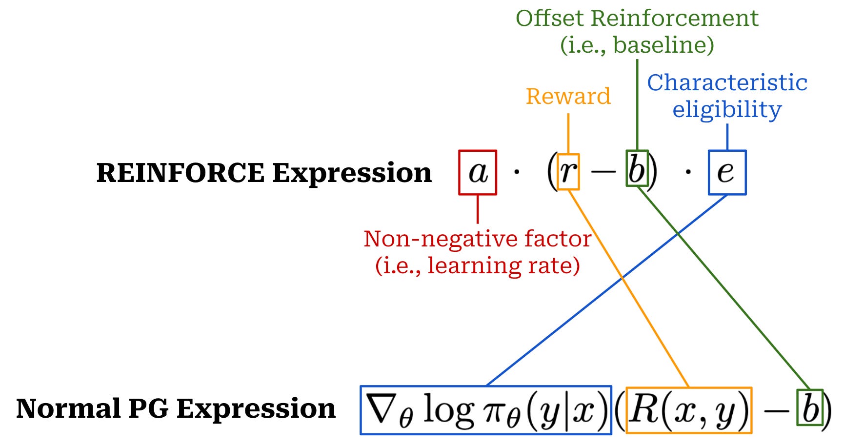
The term “offset reinforcement” is straightforward to understand. The baseline is directly subtracted from the reward in our policy gradient expression. In other words, the baseline is used to offset the reward, which is the reinforcement signal in RL (i.e., the reward determines whether actions are good or bad). The baseline is, therefore, an offset to the reinforcement signal. Unpacking the term “characteristic eligibility” requires a slightly deeper understanding of RL terminology.

“Characteristic Eligibility: This is how the learning becomes attributed per token. It can be a general value, per parameter, but is often log probabilities of the policy in modern equations.” - RLHF book

“Eligibility” is a jargon term in RL related to the credit assignment problem—or the problem of determining which specific actions contributed to the reward received by the policy. Specifically, eligibility refers to whether a particular action taken by the LLM is actually responsible for a given reward. In the policy gradient expression, credit assignment is handled by the log probabilities of actions under the policy.

Incorporating KL divergence. As with most other RL training algorithms, we also incorporate the Kullback-Leibler (KL) Divergence with respect to a reference policy—usually a prior SFT-trained checkpoint of our model—into REINFORCE. We have several different approaches for approximating KL divergence. A common approach is to approximate KL divergence as the difference in log probabilities between the policy and reference policy. Once we’ve made this approximation, the KL divergence is directly incorporated into the reward as shown below.

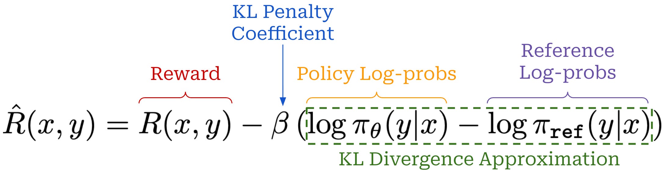
This approach of subtracting the KL penalty from the reward varies depending on the RL training algorithm or implementation. For ex ample, GRPO incorporates the KL divergence into the loss function rather than directly into the reward. Adding the KL divergence into RL regularizes the training process and allows us to ensure that our policy does not deviate significantly from the reference policy.

Efficiency & overhead. Compared to algorithms like PPO, REINFORCE has reduced overhead, as it does not require the use of a value (or critic) model to compute the advantage estimate—the average of rewards is used in place of the critic. Therefore, there are only three LLM involved in the training process (i.e., policy, reference policy, and reward model), rather than four; see below. The downside of estimating the advantage in this way is higher variance. As we will see, however, the high variance of REINFORCE is not always a problem in the domain of finetuning LLMs—this simple algorithm is actually quite effective in practice.

Key models involved in training with REINFORCE

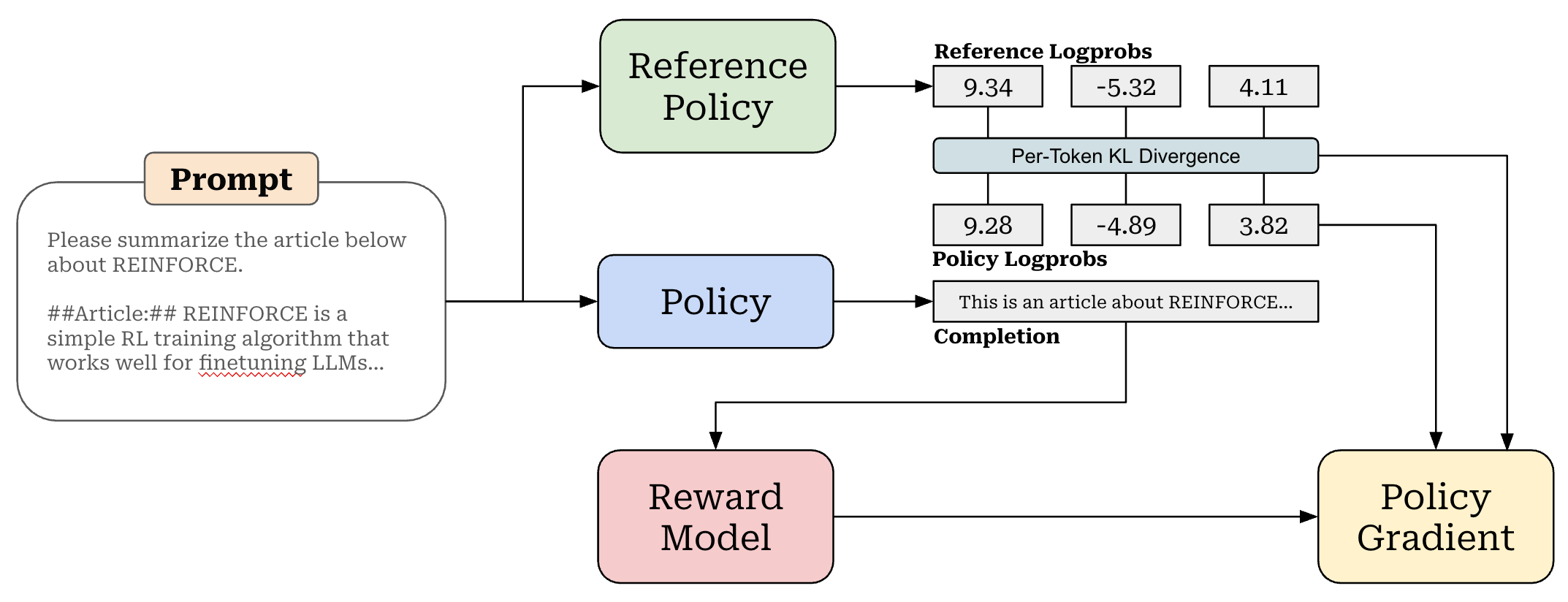
Modeling full completions. There is one final detail missing from the image above: How do we aggregate the log probabilities, KL divergences, and rewards to form the policy gradient update? One of the key distinguishing aspects of REINFORCE is that is uses a bandit formulation. The policy is trained by considering the full completion, rather than each token in the completion, as a single action.

“[REINFORCE] treats the entire model completion as a single action, whereas regular PPO treats each completion token as individual actions. Typically, only the EOS token gets a true reward, which is very sparse. Regular PPO would attribute a reward to the EOS token, whereas [REINFORCE] would attribute that EOS reward to the entire completion.” - from [5]

As we’ve learned, most LLMs are trained using an outcome reward setting, meaning that only the final <eos> token generated by the LLM is assigned a reward. However, the KL divergence is computed on the per-token basis, and—as mentioned before—the KL divergence is directly subtracted from the reward in REINFORCE. Therefore, we end up with a setup where the reward for all tokens in the completion is just the KL divergence, but the final token in the completion receives an additional reward from the reward model; see below.

Bandit formulation in REINFORCE

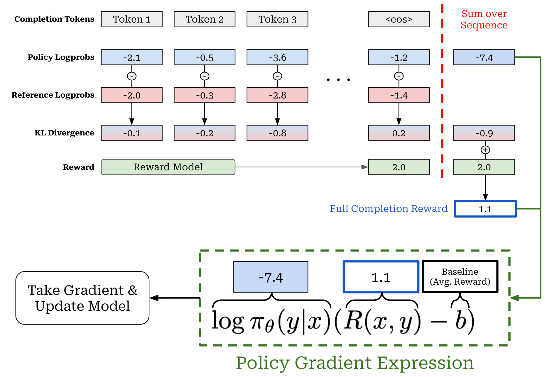
We create a completion-level (bandit formulation) reward by summing per-token KL divergences and rewards over the sequence. Similarly, we can sum token-level log probabilities to get the log probability of the completion (or trajectory)⁸. As shown above, we can then use these completion-level components to compute the policy gradient similarly to before:

1. Subtract the baseline (average reward) from the completion-level reward.

2. Multiply this difference by the completion log probability.

3. Run a backward pass to compute the final policy gradient⁹.

This process computes the policy gradient for a single prompt and completion pair, but we generally average this gradient over a batch of completions.

Pseudocode. As a final step, we will make this discussion more concrete by implementing the computation of the policy gradient for REINFORCE in basic PyTorch¹⁰. We will assume that the baseline is computed by taking an average of rewards in the batch (i.e., rather than by using a moving average) so that the entire gradient update can be outlined within a single script; see below.

import torch

# constants
kl_beta = 0.1

# batch of two completions with three tokens each
per_token_logprobs = torch.tensor(
    [
        [-12.3, -8.3, -2.3],
        [-10.0, -7.0, -3.0],
    ],
    requires_grad=True,
)
reference_per_token_logprobs = torch.tensor([
    [-11.3, -8.4, -2.0],
    [-9.5, -7.2, -2.8],
])

# compute KL divergence approximation
kl_div = per_token_logprobs - reference_per_token_logprobs
kl_div = -kl_beta * kl_div

# get reward for each completion (e.g., from reward model)
score_from_rm = torch.tensor([1.0, 0.5])

# reward is attributed to final <eos> token
per_token_reward = kl_div.clone()
per_token_reward[range(per_token_reward.size(0)), -1] += score_from_rm

# compute REINFORCE update over full sequence
entire_completion_reward = per_token_reward.sum(dim=1)
baseline = entire_completion_reward.mean().detach()

# compute advantage
advantage = entire_completion_reward - baseline

# compute loss and gradient update
reinforce_loss = -per_token_logprobs.sum(dim=1) * advantage
reinforce_loss.mean().backward()

REINFORCE Leave One Out (RLOO) [2]

In REINFORCE, we generate a single on-policy completion per prompt during training and use the rewards from these completions to form our baseline via a moving average or an average of rewards in the batch. REINFORCE leave-one-out (RLOO) [2] changes this approach by:

1. Sampling multiple (K) completions per prompt.

2. Using these multiple completions to compute the reward average separately for each individual prompt.

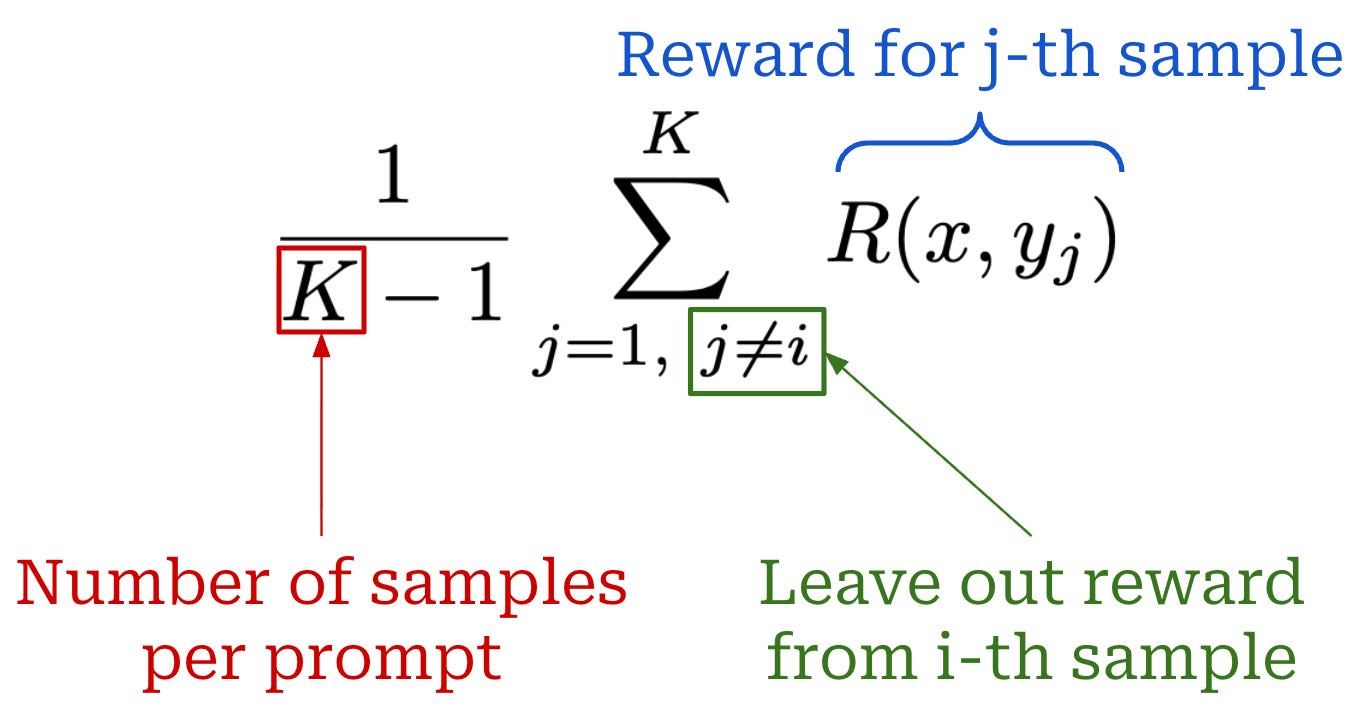
Given K completions {y_1, y_2, …, y_K} to a prompt x, RLOO defines the baseline for completion y_i as shown below, which is simply an average over all rewards for completions to prompt x excluding the completion itself y_i. We “leave out” the reward of the completion for which the policy gradient is being computed and average over the rewards of other completions to the same prompt.

Computing the baseline for RLOO

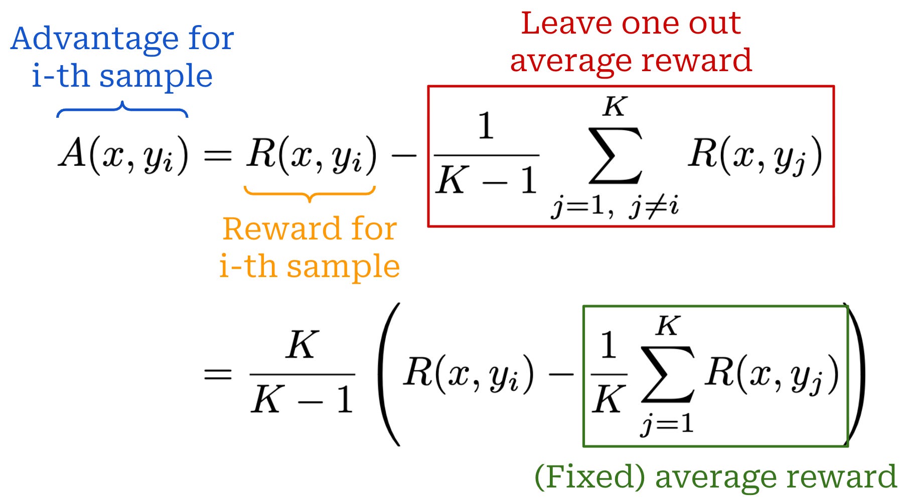
From here, we can compute the advantage estimate in RLOO by i) computing this baseline for every completion in the batch and ii) subtracting the baseline from the reward received by the completion; see below (first equation). To efficiently compute the baseline for RLOO, we can first compute a fixed average reward over the K completions and reformulate the advantage as in the second equation below. This approach allows us to compute the average reward once and avoid re-computing the leave one out average for all K completions to the prompt x.

Advantage estimate in RLOO

This modified advantage estimate can be plugged into the same policy gradient expression used by REINFORCE. Similarly to REINFORCE, RLOO uses a per-completion—as opposed to per-token—loss, and we have no learned value model. However, the leave one out baseline used by RLOO lowers variance relative to the standard REINFORCE algorithm by using multiple samples per prompt to derive the policy gradient estimate. Compared to a single-sample approach, taking multiple samples per prompt benefits training stability, speed, and performance.

“The common case of sampling one prediction per datapoint is data-inefficient. We show that by drawing multiple samples per datapoint, we can learn with significantly less data, as we freely obtain a REINFORCE baseline to reduce variance.” - from [2]

Practical usage. After the popularization of RLOO for LLMs, a great blog on this topic was published by HuggingFace [5] exploring the implementation and practical performance of RLOO. This analysis extends authors’ prior work on correctly implementing and tuning PPO-based RLHF on summarization tasks [6]—OpenAI’s TL;DR summarization dataset in particular. In [5], these results are extended by training Pythia 1B and 6.9B models with RLOO, starting from the same SFT checkpoints and reward models from [6]. Models are evaluated by comparing their output to a reference summary with a GPT-4 judge; see below.

(from [5])

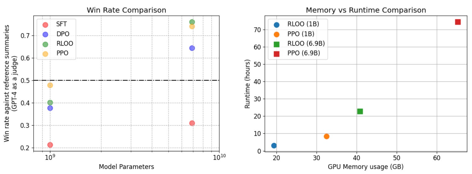
As we can see, RLOO uses 50-70% less memory than PPO and runs 2-3× faster. These savings increase with the size of the model. In addition to these gains in efficiency, RLOO performs competitively to PPO and consistently outperforms offline algorithms like DPO. These results demonstrate the key value proposition of RLOO (and REINFORCE)—these algorithms maintain the performance benefits of online RL algorithms while being simpler to implement and less costly to run.

Pseudocode. To implement RLOO, we can modify our original REINFORCE example as shown below. Here, we assume that three completions are sampled per prompt (i.e., K = 3) and that our batch is composed of three prompts. For more production-ready code, both REINFORCE and RLOO are also supported within the volcano engine reinforcement learning (verl) library [7]; see here.

import torch

# constants
K = 3  # completions per prompt
kl_beta = 0.1

# batch of three prompts with three completions each
per_token_logprobs = torch.tensor(
    [
        # prompt 1
        [
            [-12.3, -8.3, -2.3], # completion 1
            [-10.0, -7.0, -3.0], # completion 2
            [-10.5, -12.2, -9.1], # completion 3
        ],

        # prompt 2
        [
            [-11.0, -10.3, -1.3],
            [-11.1, -11.1, -0.8],   
            [-8.2, -11.9, -0.1],        

        ],
        
        # prompt 3
        [
            [-1.8, -2.1, -0.2],
            [-0.7, -3.5, -0.1],
            [-1.0, -2.2, -1.1],
        ],
    ],
    requires_grad=True,
)
reference_per_token_logprobs = torch.tensor([
    [
        [-11.8, -8.4, -2.3], 
        [-10.1, -7.2, -3.1],
        [-10.3, -12.9, -9.1],
    ],
    [
        [-11.8, -9.7, -1.3],
        [-12.3, -11.9, -0.2],
        [-8.1, -12.0, -0.5],
    ],
    [
        [-2.7, -2.0, -1.2],
        [-0.7, -3.6, -0.2],
        [-0.7, -1.2, -0.9],
    ],
])

# compute KL divergence approximation
kl_div = per_token_logprobs - reference_per_token_logprobs
kl_div = -kl_beta * kl_div

# reward for each completion (grouped by prompt)
score_from_rm = torch.tensor([
    [1, 2, 3], # rewards for completions to prompt 1
    [2, 3, 4], # rewards for completions to prompt 2
    [3, 4, 5], # rewards for completions to prompt 3
]).float()

# reward attributed to final <eos> token
per_token_reward = kl_div.clone()
per_token_reward[:, :, -1] += score_from_rm

# compute full sequence reward
entire_completion_reward = per_token_reward.sum(dim=-1)

# compute RLOO baseline in vectorized fashion
baseline = (
    entire_completion_reward.sum(dim=-1)[:, None]
    - entire_completion_reward
) / (K - 1)
baseline = baseline.detach()

# compute advantage and loss
advantage = entire_completion_reward - baseline
rloo_loss = -per_token_logprobs.sum(dim=-1) * advantage
rloo_loss.mean().backward()

Back to Basics: Revisiting REINFORCE Style Optimization for Learning from Human Feedback in LLMs [3]

“We posit that most of the motivational principles that led to the development of PPO are less of a practical concern in RLHF and advocate for a less computationally expensive method that preserves and even increases performance.” - from [3]

Although PPO is the de facto RL optimizer for RLHF, authors in [3] argue that the original motivations for PPO (i.e., avoiding large and unstable policy updates) are less relevant in the context of LLMs. Instead, we can use simpler RL optimizers—REINFORCE in particular—to save on compute and memory costs without sacrificing performance. In particular, we learn that aligning LLMS with a basic REINFORCE algorithm can achieve results that match or exceed those of PPO-based RLHF, as well as other algorithms like DPO and RAFT. This paper was a key contribution that popularized the use of simpler RL optimizers for LLMs.

LLMs versus DeepRL. The crux of the argument in [3] revolves around the fact that LLM finetuning is a unique setting for RL that differs significantly from the traditional DeepRL setting in which algorithms like PPO were proposed. The most notable difference between these two settings is that LLMs are not trained with RL from scratch. Rather, we are finetuning an LLM that has already undergone extensive pretraining. This difference has two key implications:

• The risk of policy updates with catastrophically large variance is lower in LLM finetuning relative to the traditional DeepRL setting.

• The LLM finetuning setting has less of a need for regularizing the learning process relative to the traditional DeepRL setting.

We can concretely test this hypothesis by tweaking the settings of PPO. Namely, most implementations of PPO use Generalized Advantage Estimation (GAE) [4] to estimate the advantage function. The details of GAE are beyond the scope of this post. However, GAE contains the λ ∈ [0.0, 1.0] hyperparameter that can be used to control the tradeoff between bias and variance in the advantage estimate.

(from [3])

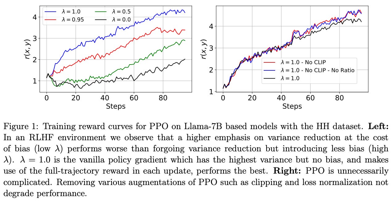
Lowering λ reduces variance at the cost of increased bias, but this is a worthwhile tradeoff for domains—like DeepRL—with excessive variance in policy updates. As shown above, optimal performance in LLM alignment is achieved with a setting of λ = 1.0, which induces maximum possible variance in the policy gradient. Such a finding indicates that the level of variance in policy updates observed for LLM alignment is not detrimental to the LLM’s learning process.

“Large off-policy updates in our optimization regime are rare and do not have catastrophic effects on learning as they do in traditional DeepRL.” - from [3]

Effective action space. In addition to high variance, one complicating factor of RL training is the presence of a large action space. If there are many possible actions for the policy to take and rewards from these actions are noisy, learning a high-quality policy is difficult. Theoretically, the action space of an LLM is very large—it includes all completions that the LLM can generate for a given prompt.

(from [3])

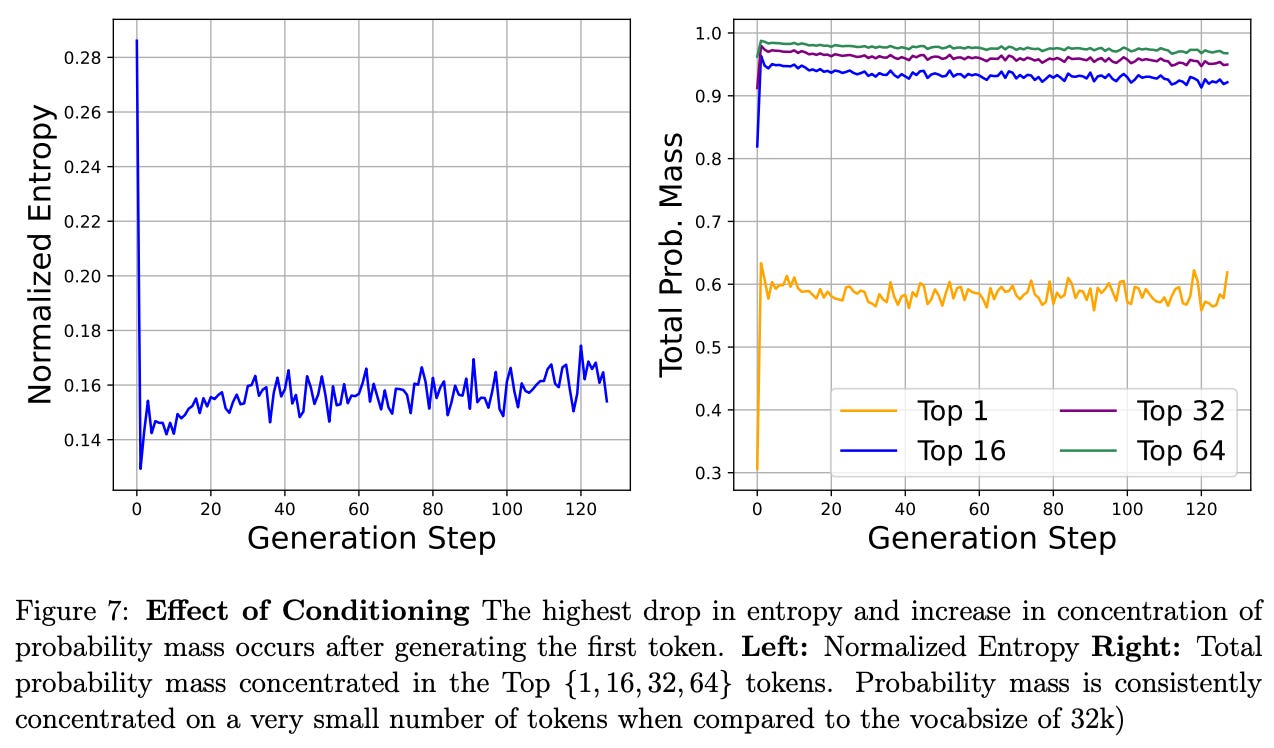
Practically speaking, however, the effective action space of an LLM—the set of completions that the model is likely to generate—is actually quite small. When an LLM is performing generation, this process is conditioned upon the prompt provided to the LLM, which is shown in [3] to be a strong conditioning.

(from [3])

More specifically, we see in the figure above that probability mass in an LLM’s completions is highly-concentrated amongst a small number of tokens after the first step of the generation process (i.e., the first token that is outputted). Such an observation demonstrates that an LLM’s prompt provides strong conditioning for the generation process, which makes the mode’s effective action space quite small.

From PPO to REINFORCE. Given that variance is less of a concern for LLMs, authors in [3] perform RLHF experiments that use much simpler REINFORCE and RLOO algorithms as the RL optimizer in place of PPO. REINFORCE and RLOO make significant changes to the RL formulation used in PPO. Namely, PPO uses a per-token MDP formulation, while both REINFORCE and RLOO adopt a bandit formulation—the entire completion is modeled as a single action.

“We show that the modeling of partial sequences is unnecessary in this setting where rewards are only attributed to full generations… it is more appropriate and efficient to model the entire generation as a single action with the initial state determined by the prompt.” - from [3]

In addition to being simpler than the MDP formulation, modeling the full generation as a single action preserves the LLM’s performance and even speeds up learning, indicating that formulating each token as its own action is an unnecessary complexity in an outcome reward setting.

Experimental setup. Experiments in [3] are conducted on the TL;DR summarize and Anthropic HH datasets with Pythia-6.9b and Llama-7b models. Both reward models and policies are initialized using a model checkpoint obtained by running SFT on a curated dataset of high-quality completions for each respective dataset. During RL, training prompts are sampled from the SFT dataset. For evaluation, authors report each model’s average reward—from the fixed reward model used for RL training—on a hold out test set, as well as win-rates against GPT-4 using the AlpacaFarm framework (i.e., open-ended evaluation on chat-style prompts).

(from [3])

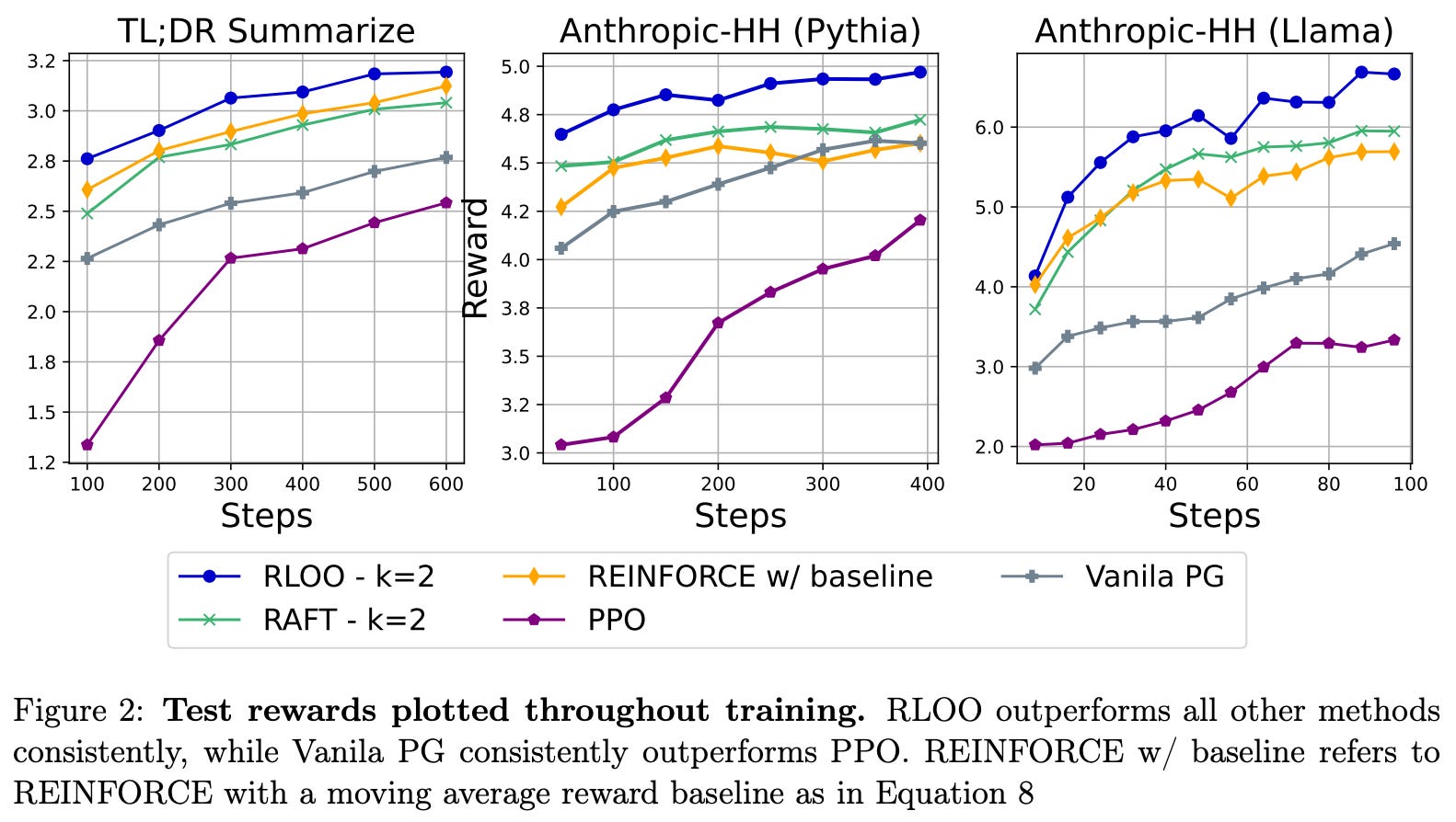
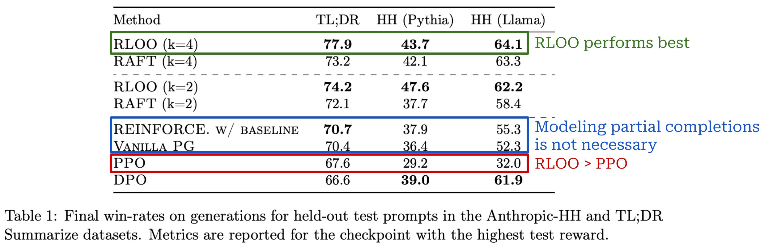
Is REINFORCE effective? As shown above, both REINFORCE and RLOO—in addition to being less memory intensive due to their lack of a learned critic model—consistently outperform PPO, confirming that modeling partial sequences is unnecessary for the RLHF setting in [3]. RLOO is also found to be more sample efficient than the RAFT algorithm [9]—given the same number of on-policy samples generated during training, RLOO tends to achieve better performance; see below.

(from [4])

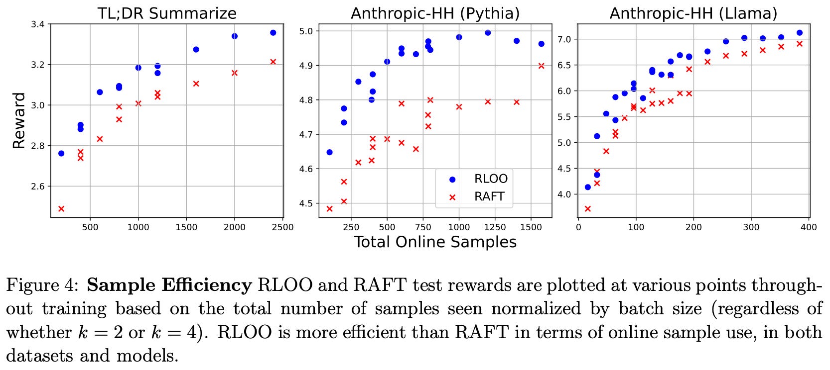
This finding holds true for all models and data tested in [3]. The superior sample efficiency of RLOO makes intuitive sense given that all samples—even those with poor or negative reward—are used during training. In contrast, RAFT filters samples based on their reward and only trains on those with the best rewards.

When we evaluate models in terms of simulated win-rates on AlpacaFarm, many of the results above continue to be true, but we can compare the performance of each technique in a more human-understandable manner. As shown below, the best performance is consistently achieved with RLOO, and both REINFORCE and RLOO consistently outperform PPO. Notably, RLOO—with four on-policy samples per prompt—outperforms PPO by an absolute increase in win-rate of 10.4% and 14.5% for TL;DR and HH datasets. When used to align Llama, RLOO sees an even larger absolute win-rate improvement of 32.1% over PPO.

(from [3])

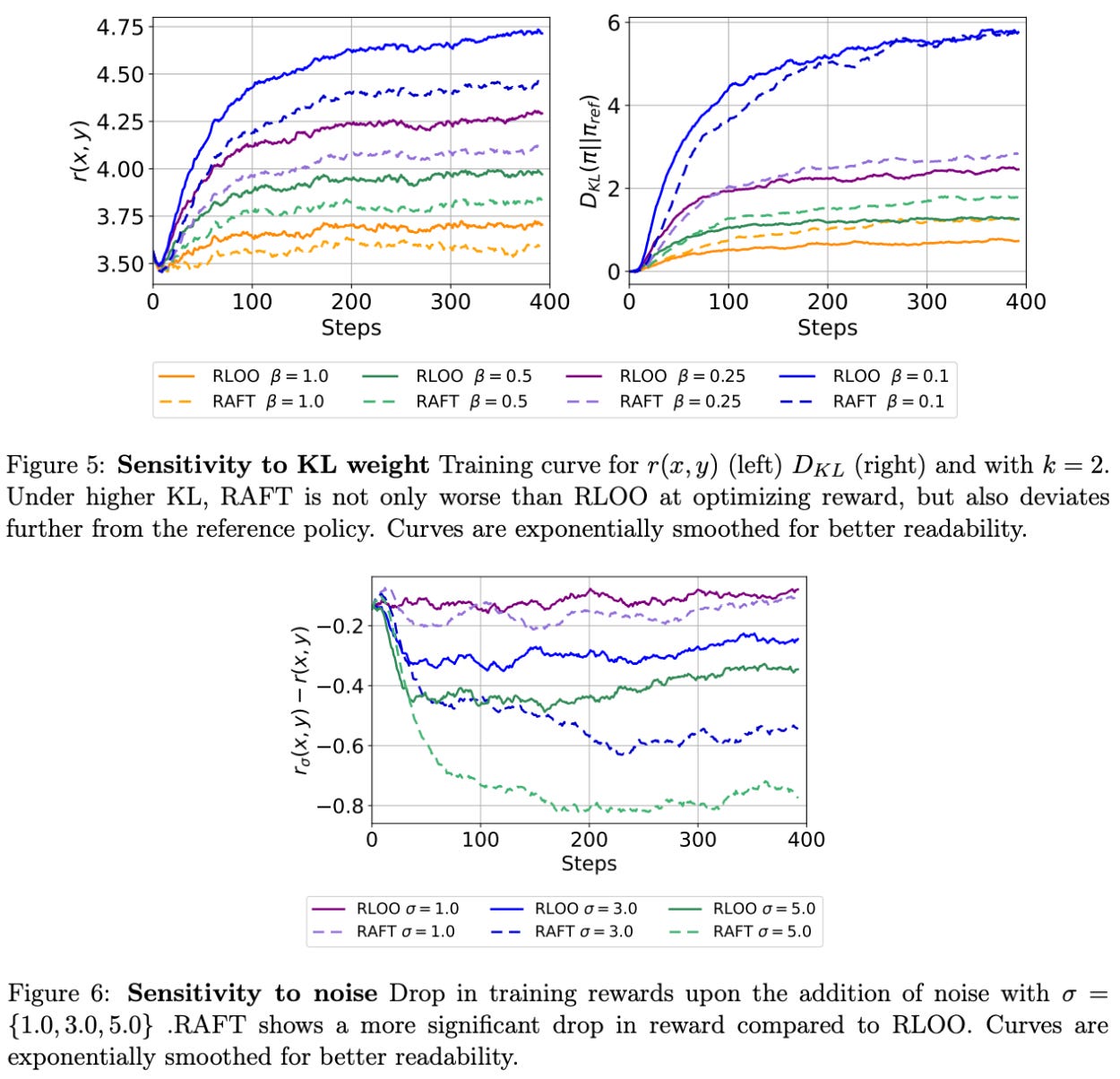
Improved robustness. Authors in [3] conclude by studying the robustness of RLOO relative to RAFT in two areas:

• How does increasing the β term for KL divergence impact performance?

• How does adding noise to the reward estimate impact performance?

Interestingly, RLOO is found to be noticeably more robust to noise relative to RAFT; see below. When increasing β, RAFT performs worse than RLOO and produces a policy with a larger KL divergence relative to the reference policy. Additionally, the performance of RAFT sees a larger negative impact from noisy reward estimates relative to RLOO. Such degraded robustness to noise is caused by the fact that RAFT only trains on the highest-reward completions, leading any perturbation to reward estimates to significantly impact training.

(from [3])

Conclusion

We now have a foundational understanding of RL for LLMs that spans from basic terminology to functional implementations of online RL algorithms. Most work on RL training for LLMs uses actor-critic algorithms like PPO as the underlying optimizer. But, these algorithms introduce complexity and overhead to reduce the variance of policy gradients. In the context of LLMs, we have learned that much simpler online RL algorithms are available! REINFORCE and RLOO adopt a completion-level bandit setup for RL and normalize rewards using either:

• The average of rewards during training (for REINFORCE), or

• The average of rewards for other completions to a prompt (for RLOO).

Because they estimate the value function in this way, neither REINFORCE or RLOO require a learned critic, which reduces memory overhead and speeds up the training process. If we want to avoid the complexity of algorithms like PPO, these simpler online RL algorithms offer an effective alternative, rather than immediately turning to approaches that are completely offline or RL-free.

New to the newsletter?

Hi! I’m Cameron R. Wolfe, Deep Learning Ph.D. and Senior Research Scientist at Netflix. This is the Deep (Learning) Focus newsletter, where I help readers better understand important topics in AI research. The newsletter will always be free and open to read. If you like the newsletter, please subscribe, consider a paid subscription, share it, or follow me on X and LinkedIn!

Bibliography

[1] Williams, Ronald J. “Simple statistical gradient-following algorithms for connectionist reinforcement learning.” Machine learning 8.3 (1992): 229-256.

[2] Kool, Wouter, Herke van Hoof, and Max Welling. “Buy 4 reinforce samples, get a baseline for free!.” (2019).

[3] Ahmadian, Arash, et al. “Back to basics: Revisiting reinforce style optimization for learning from human feedback in llms.” arXiv preprint arXiv:2402.14740 (2024).

[4] Schulman, John, et al. “High-dimensional continuous control using generalized advantage estimation.” arXiv preprint arXiv:1506.02438 (2015).

[5] Costa Huang, Shengyi, et al. “Putting RL back in RLHF” https://huggingface.co/blog/putting_rl_back_in_rlhf_with_rloo (2024).

[6] Huang, Shengyi, et al. “The n+ implementation details of rlhf with ppo: A case study on tl; dr summarization.” arXiv preprint arXiv:2403.17031 (2024).
[7] Sheng, Guangming, et al. “Hybridflow: A flexible and efficient rlhf framework.” Proceedings of the Twentieth European Conference on Computer Systems. 2025.

[8] Lightman, Hunter, et al. “Let’s verify step by step.” The Twelfth International Conference on Learning Representations. 2023.

[9] Dong, Hanze, et al. “Raft: Reward ranked finetuning for generative foundation model alignment.” arXiv preprint arXiv:2304.06767 (2023).

1. In other words, the output of our policy is not just a discrete action. Rather, it is a probability distribution over a set of possible actions. For example, LLMs output a probability distribution over the set of potential next tokens.

2. Additionally, we can have a finite or infinite-horizon setup in this return. However, in the context of LLMs, we usually assume a finite-horizon setup (i.e., the LLM does not continue generating tokens forever).

3. Here, we use gradient ascent (as opposed to descent) because we are trying to maximize a function. However, gradient ascent and descent are nearly identical. The only change is whether we subtract—if minimizing a function in gradient descent—or add—if maximizing a function in gradient ascent—the gradient to our model’s parameters.

4. Process supervision is possible and has been explored in research on large reasoning models (LRMs), but it is less common than the outcome reward setting.

5. Additionally, adding baselines to the policy gradient does not bias our gradient estimate. This fact can be proven by using the EGLP lemma, which also mandates that the baseline must only depend on the state s_t.

6. By “head”, we mean an extra small layer added to the end of the LLM that is trainable.

7. The “actor” refers to the LLM—or the model that is taking actions—and the “critic” refers to the value model. The value model is called a critic due to the fact that it is predicting the reward associated with each action (i.e., effectively critiquing the action).

8. This stems from basic concepts in language modeling. Namely, we can take the product of probabilities for all tokens in a completion (or the sum of log probabilities) to get the probability of the full completion.

9. Our policy gradient term contains the gradient of log probabilities, but we have access to log probabilities (not the gradient of log probabilities) in our example. So, we need to take the gradient of these log probabilities—usually by running loss.backward() in PyTorch—to get the final policy gradient.

10. This implementation, as well as our later implementation of RLOO, is just a modified version of the code from this blog post.