
Continual Learning with RL for LLMs
Exploring the impressive continual learning capabilities of RL training...

Continual learning, which refers to the ability of an AI model to learn from new tasks and data over time, has become a popular topic in the discussion of Artificial General Intelligence (AGI). Put simply, general intelligence should be adaptable, which has led some to believe that continual learning abilities are a prerequisite for AGI. The reasoning behind this argument is clear—dynamically adapting to arbitrary tasks (i.e., “on-the-job” learning) is a common trait of humans—but rigorously studying this concept is hard. In the real world, continual learning is unstructured, noisy, and open-ended. In order to make meaningful progress, we must transform this complex process into a more structured empirical setting.
“LLMs don’t get better over time the way a human would. The lack of continual learning is a huge huge problem. The LLM baseline at many tasks might be higher than an average human’s. But there’s no way to give a model high level feedback. You’re stuck with the abilities you get out of the box.” - Dwarkesh Patel
To do this, we can pull from decades of prior research on the topic of continual learning for neural networks [10]. Although much of this work predates LLMs, such research provides a foundational understanding of continual learning and addresses key questions that are still relevant in the modern era:
Why is continual learning difficult?
How should we structure continual learning experiments?
Which techniques are effective in practice?
In this overview, we will bridge decades of continual learning research with more recent work on LLMs to develop a comprehensive perspective on the topic. While core concepts (e.g., catastrophic forgetting, experimental frameworks, method categories, etc.) carry over directly, continual learning for LLMs is unique because of scale. Even simple techniques become complex systems problems when considering the vast data and prior knowledge of modern LLMs. As we will learn, however, continual learning is not disjoint from current LLM research. Rather, existing post-training techniques—especially on-policy reinforcement learning (RL)—can naturally mitigate catastrophic forgetting, providing hope that continual learning is within reach given the current trajectory of LLM research.
Basics of Continual Learning
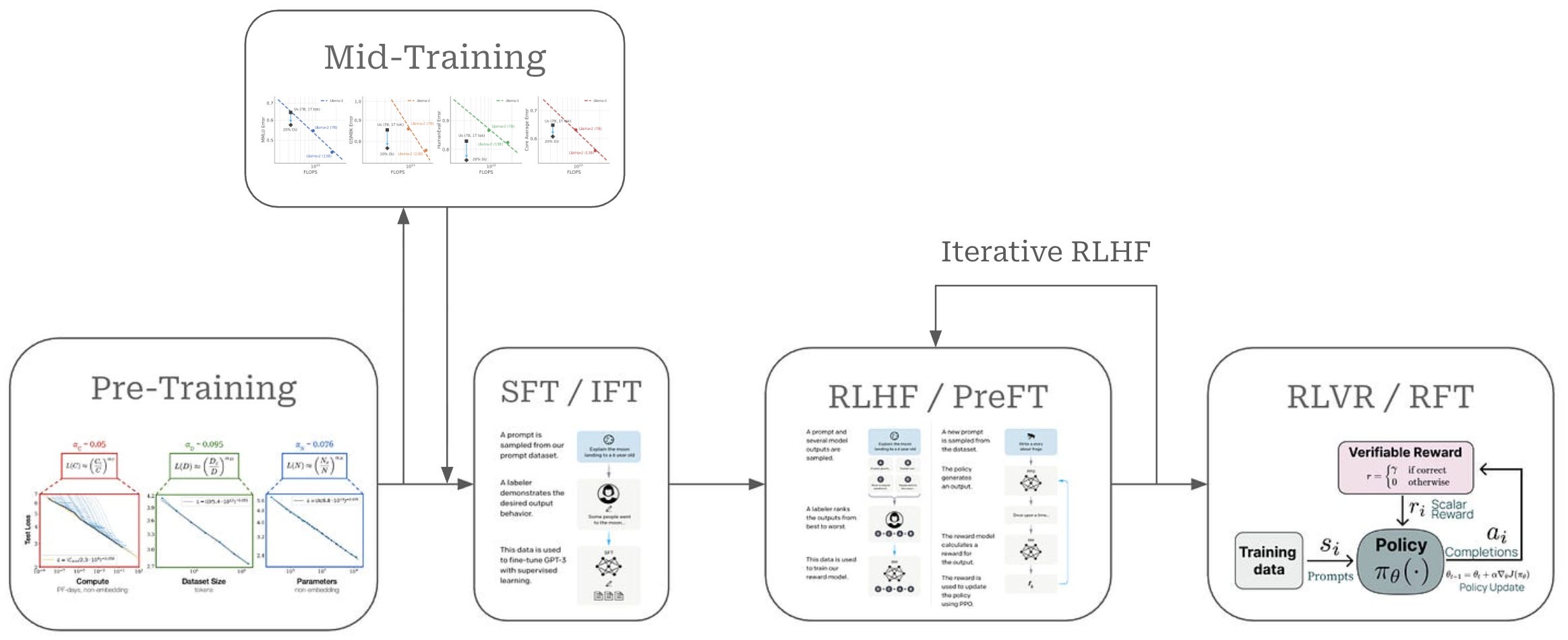
The continual learning paradigm is starkly different from how neural networks are typically trained: for several epochs over a large, fixed dataset. Modern LLM training pipelines already include a mix of offline and more iterative components. Some stages (e.g., pretraining) closely resemble classical offline training, while others (e.g., iterative RLHF or online RL) begin to capture aspects of continual learning. In this section, we will develop a foundational understanding of continual learning—how it is studied, common experimental frameworks, and the major categories of methods proposed for both LLMs and neural networks more broadly.
Catastrophic Forgetting
Historically, the difficulty of continual learning does not stem from a model’s inability to learn new tasks, but rather its tendency to degrade in performance on old tasks when training on new data. For example, running supervised training of an LLM over a new dataset will quickly enhance its in-domain performance. But, the same model may significantly deteriorate in its performance across general benchmarks or tasks that were observed previously in the training process.
“Disruption of old knowledge by new learning is a recognized feature of connectionist models with distributed representations. However, the interference is sometimes described [as] mild or readily avoided. Perhaps for this reason, the interference phenomenon has received surprisingly little attention, and its implications for connectionist modeling of human cognition have not been systematically explored.” - from [10]
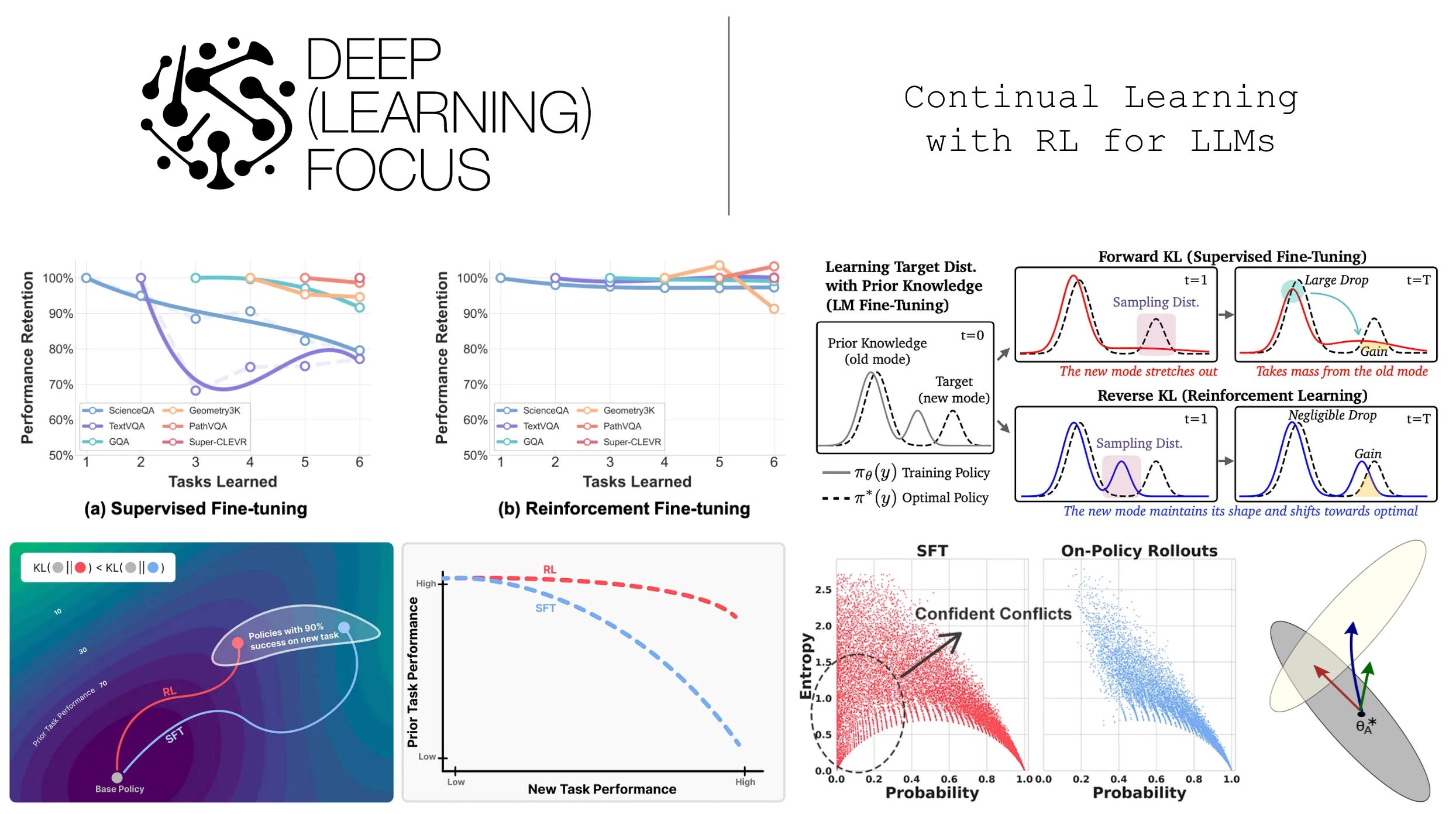
In continual learning research, this phenomenon is referred to as “catastrophic forgetting”1 [11]. Training our model over new data tends to come at the cost of a significant—or catastrophic—degradation in performance on other tasks. The goal of research in this area is, therefore, to mitigate catastrophic forgetting. The figure below helps us to better understand this phenomenon. Here, a model is initially trained on task A (grey) before being exposed to a new task (yellow).
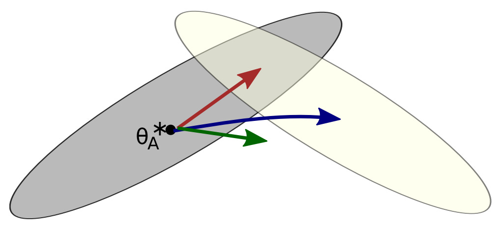
The three arrows in the figure depict three possible solutions that can emerge when trying to solve this continual learning problem. The red arrow depicts a solution that performs well on both tasks, while the blue and green arrows perform well on only the new task or neither task, respectively. Put simply, the goal of continual learning is to develop techniques that reliably follow the red arrow. More specifically, an effective continual learning system should both:
Perform well on new tasks to which it is exposed.
Maintain comparable (or better) levels of performance on prior tasks.
As we will see throughout this overview, these two objectives are usually at odds—we are constantly balancing general capacities with new tasks. Simply specializing our model to each new incoming task is not a valid approach because new tasks will always continue to emerge in a real-world setting. We must maintain the model’s generality while maximizing adaptability to arbitrary future tasks.
Experimental Frameworks for Continual Learning
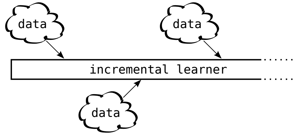
There are many continual learning variants that have been studied in the literature; e.g., continual learning, lifelong learning, incremental learning, streaming learning, and more. Despite the many variants of continual learning that exist, all of these variants share the same sequential nature of the training process—the model is exposed to new data over time and cannot return to data from the past (unless explicitly stored in a buffer) when learning from new data; see below.
Non-IID data. First, we must consider the kind of data being exposed to our model. If the incremental data over which the model is trained is sampled from the model’s training distribution, then training on this data is unlikely to cause forgetting. This setup resembles a continued training approach, which is used frequently for LLM pre and post-training. However, if the incremental data is non-IID—or sampled from a distribution that is new or different from the training data distribution—then catastrophic forgetting becomes very likely; see below.
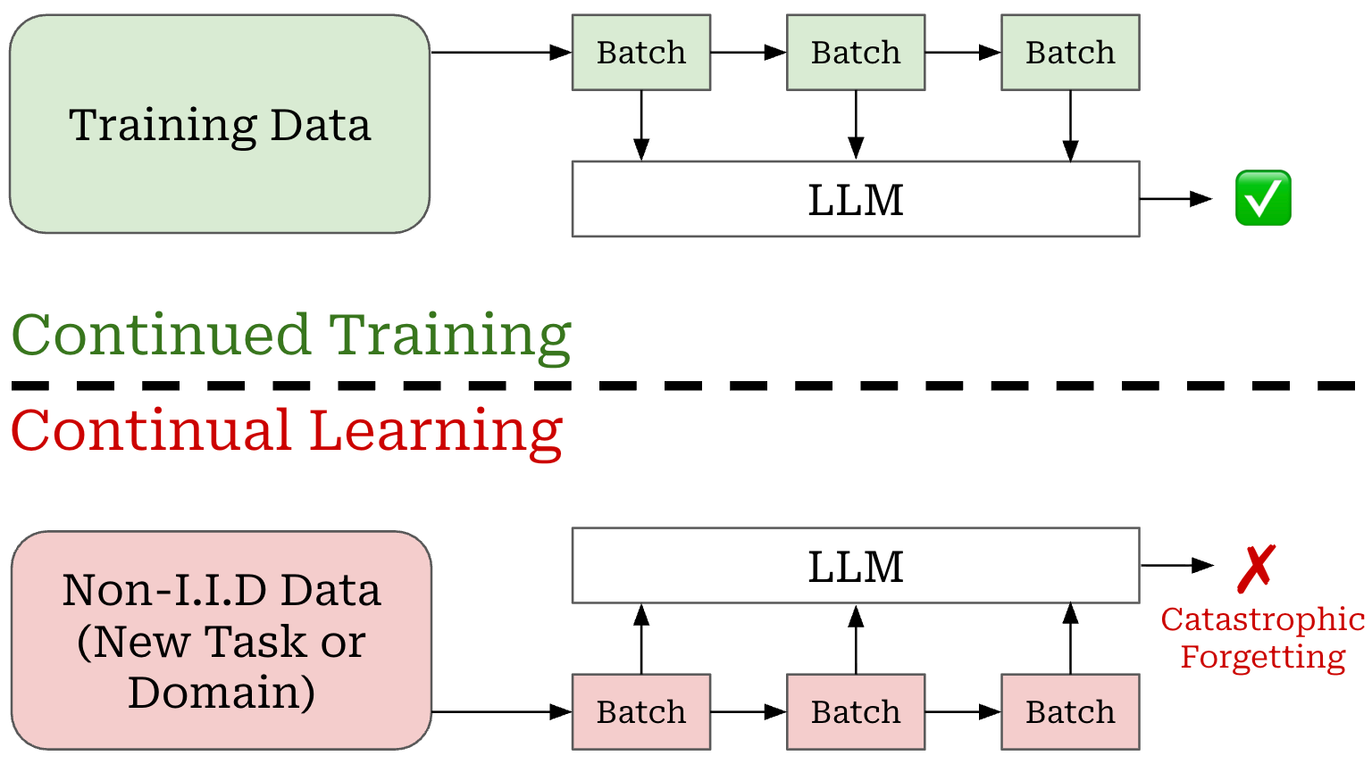
For this reason, most experimental frameworks for continual learning assume the use of non-IID data. For example, when training an image classification model, we can derive incoming data from previously unseen classes. Similarly, we can continually train an LLM on an unseen task. In both cases, we expose the model to an unseen or different distribution of data that can induce catastrophic forgetting.
Data increments. We now need to understand the different approaches for exposing data to the model during continual learning. The most common sequential learning setup is a batch-incremental learning approach, where entire batches of data are passed to the model sequentially. These batches can be arbitrarily large (e.g., an entire new dataset or task) and the model usually trains on each batch of data before moving on to the next batch; see below.
Formally, we have a sequence of T tasks, each with an associated dataset or batch {D_1, D_2, …, D_T}. The model is sequentially trained on each task (i.e., one-by-one and in order), leading to a sequence of T models throughout the continual learning process. When training on a new task, we do not have access to prior tasks’ data. The simplest variant of batch-incremental learning is a domain adaptation setup where T = 1. For this setup, a pretrained model is trained on data from only a single new domain. The goal of continual learning in this scenario is the same, but the model only undergoes one stage of adaptation.
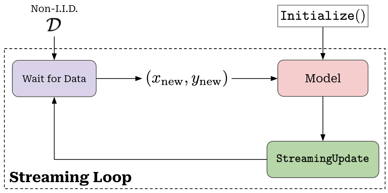
The batch-incremental framework may not always be realistic, as our model may receive data in much smaller increments. For these cases, a streaming learning setup may be more appropriate. Streaming learning uses brief, online updates (i.e., one or a few forward and backward passes) for each piece of incoming data, forcing learning of new data to happen in real-time; see below.
In contrast, batch-incremental learning setups usually perform a full, offline training procedure (i.e., several epochs of training) over each batch of incoming data. Although streaming and incremental learning setups are quite different, we can interpolate between these two approaches by:
Changing the amount of data passed to the model at each phase of sequential learning (e.g., single example, batch of examples, entire dataset, etc.).
Restricting the number of model updates at each sequential learning phase (e.g., single update, multi-update, full epoch, multi-epoch, etc.).
Multi-task learning. In order to determine if a continual learning technique is performing well, we need a baseline to which our models can be compared. A common baseline is joint (multi-task) training, where the model has access to all T tasks and can perform offline training over all of the data. Joint training over all data is the best possible training setup and allows us to understand the ceiling in performance that we are aiming to match via continual learning.
Which setup is best? In this overview, we will study a variety of continual learning papers in the LLM domain. Most of these papers adopt some variation of batch-incremental learning, where each batch is a new task that the LLM must learn. The domain-adaptation setup, in which a base LLM is trained over a single new task, is also common. These setups are useful for testing the tendency of LLMs to catastrophically forget, but one could argue that such a task-incremental setup does not reflect how LLMs would continually learn in the real world. For this reason, no one continual learning setup is the best. Rather, we should modify our experimental configuration within the frameworks outlined above such that the practical setting we are trying to test is most accurately reflected.
Common Techniques for Continual Learning
Now that we have a basic understanding of continual learning, we can overview some of the key categories of techniques for mitigating catastrophic forgetting. We will cover continual learning approaches in general, as well as highlight the methods that have been used in recent continual learning work with LLMs.
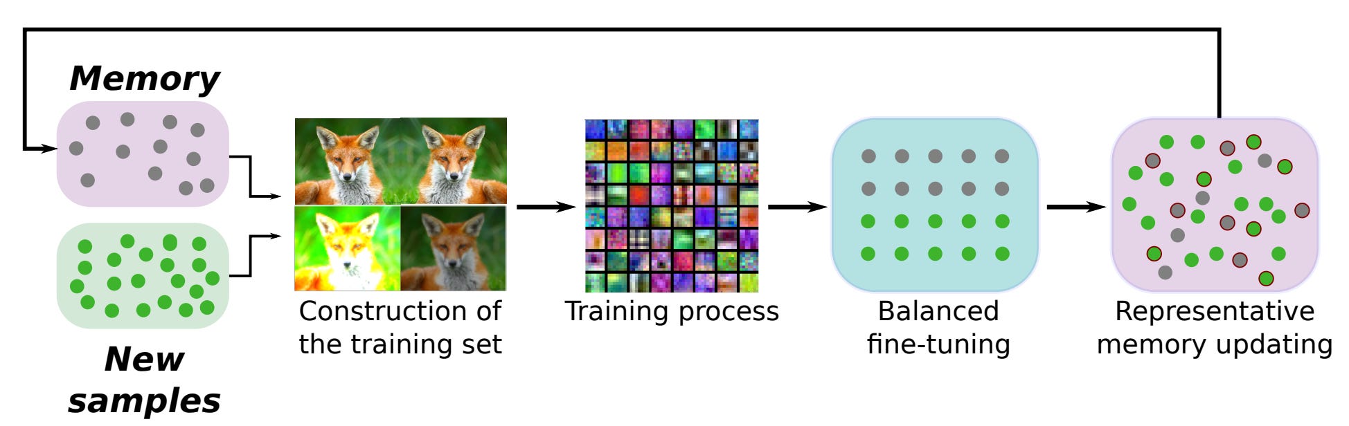
Replay mechanisms (depicted above) are a simple and effective technique for continual learning that maintain a buffer of prior data over which to train the model. Before being included in the replay buffer, samples usually undergo a selection process (e.g., based on importance or diversity) [14] to ensure that the buffer contains high-quality, representative samples and is not too large. The entire replay buffer can also be quantized or compressed to reduce memory [15]. In cases where data cannot be explicitly stored inside of a replay buffer, we can also train or maintain a generative model to replay synthetic examples [16, 17].
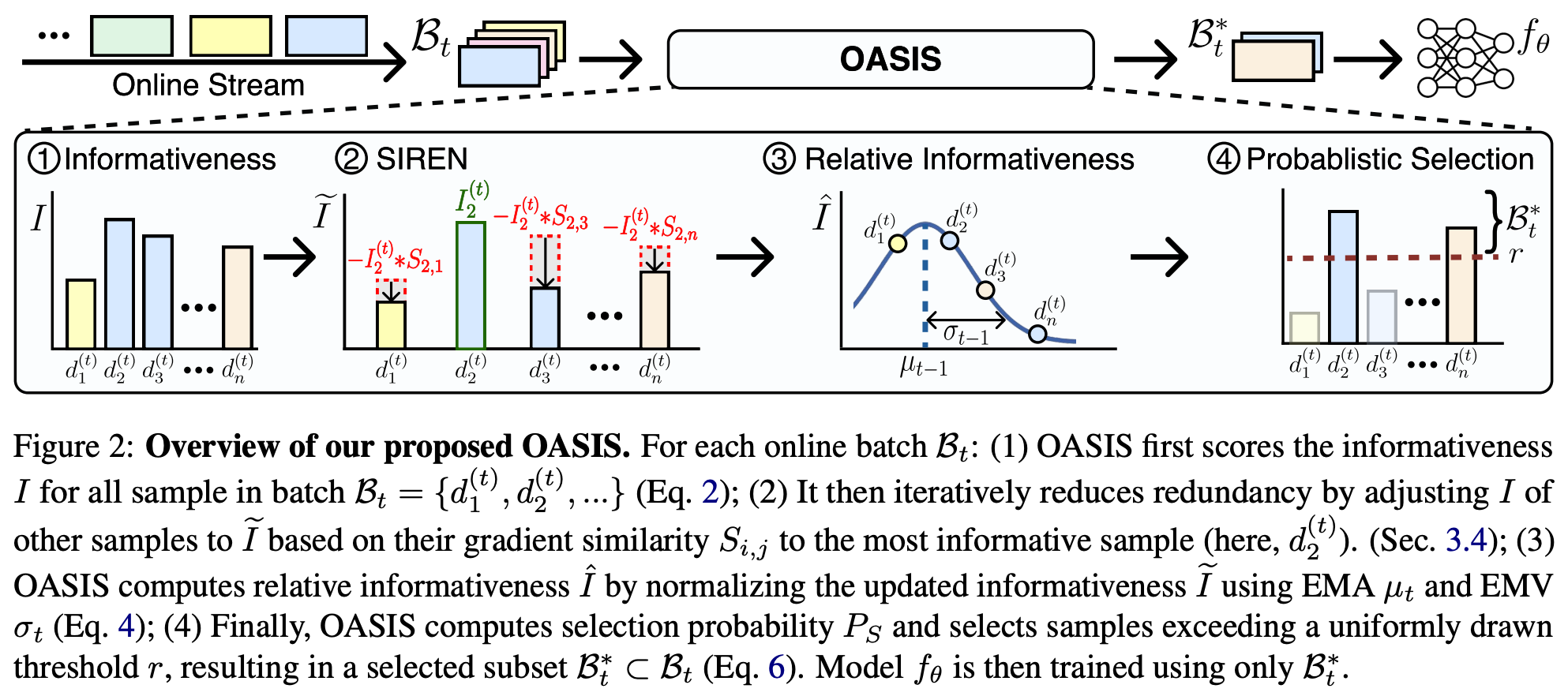
Although replay buffers are one of the most simple and effective techniques for continual learning, applying them in the LLM domain is less straightforward. Namely, LLMs have a vast amount of prior training data and, in many cases, this data is not openly available. Therefore, constructing a replay buffer that captures the general capabilities of an LLM is non-trivial. However, several works have recently explored the use of replay buffers for continual post-training. For example, instruction tuning data has a more manageable volume, allowing a replay buffer to be constructed by retaining the most important or informative data throughout the continual post-training process [30, 31]; see above.
Knowledge distillation [18] can be used to mitigate catastrophic forgetting by ensuring that a model’s representations do not drift during the continual learning process. In their simplest form, distillation-based continual learning techniques just combine the training loss on new data with a distillation loss with respect to prior model outputs [19]; see above. Many variants of this approach have been proposed [12, 20, 22]. We should also note that these techniques are not mutually exclusive; e.g., replay buffers can be combined with a distillation loss [13].
Regularization in various forms can be helpful for continual learning. In fact, knowledge distillation can even be considered a form of regularization. Researchers have explored constraining weight updates for subgroups of parameters—usually the most important parameters for a task [11, 21]—or increasing plasticity for select parameters [23]. We can also regularize the output distribution of the model by applying a KL divergence—similar to the use of KL to regularize the RL training objective—and even simple changes like lowering the learning rate have been found to reduce forgetting [2]. Model merging has also been applied in tandem with explicit regularization to reduce catastrophic forgetting in LLMs [29].
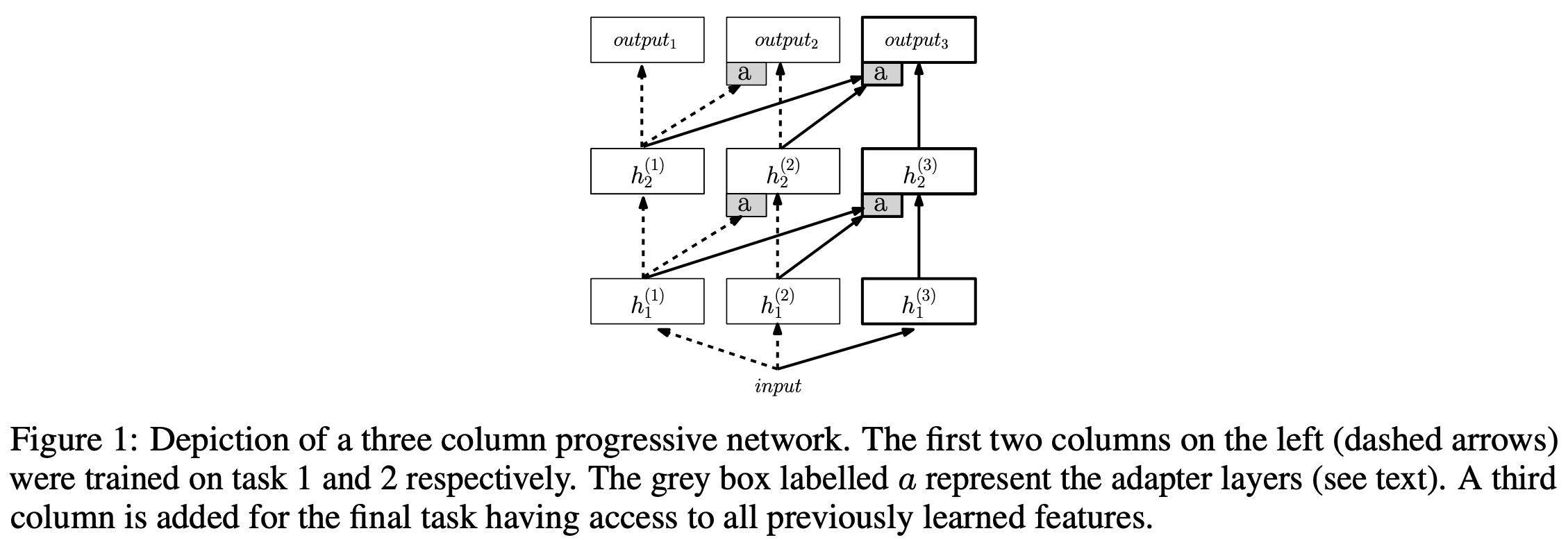
Architectural approaches have also been explored for continual learning that dynamically adapt the model’s architecture to handle incoming data. For example, new modules can be added to a neural network to handle new groups of data [24]; see above. Given the popularity of LoRA for LLMs, recent work has explored using LoRA modules as an architectural extension for learning new information during continual learning [26, 27]; see below. Mixture-of-Experts architectures for LLMs have also been shown to be better at avoiding catastrophic forgetting [28].
Further reading. We have now seen a comprehensive, high-level overview of the continual learning techniques that exist, but the literature is vast and dates all the way back to the 1980s (if not earlier)! The resources linked below will be helpful for developing a deeper understanding of continual learning research:
A broad overview of the categories of continual learning techniques.
A deep dive on streaming learning techniques.
A survey on continual learning for modern generative models.
Continual Learning for LLMs
“Surprisingly, without any data replay, continual post-training with RFT can achieve comparable performance with that of multi-task training, which is not achievable even when equipping SFT with continual learning strategies.” - from [1]
We will now take a look at several papers that study the topic of continual learning in the context of LLMs. Instead of focusing on continual learning techniques, however, these papers adopt standard LLM training methodologies—supervised finetuning (SFT) and reinforcement learning (RL) in particular—and analyze their natural ability to avoid catastrophic forgetting. Although SFT tends to not perform well for continual learning, RL is found to be shockingly robust to forgetting, even without employing explicit continual learning techniques (e.g., replay buffers or regularization). Given the current popularity and impact of RL in training frontier models, this inherent ability to handle continual learning makes RL an important tool for the creation of generally intelligent systems.
More on SFT and RL
To understand the different behaviors of SFT and RL in the continual learning setting, we need to gain a deeper understanding of the learning mechanisms that underlie these algorithms. For a full overview of each technique, please see the following resources:
As we will see, all of the papers in this overview adopt a reinforcement learning with verifiable rewards (RLVR) setup with GRPO as the RL optimizer.
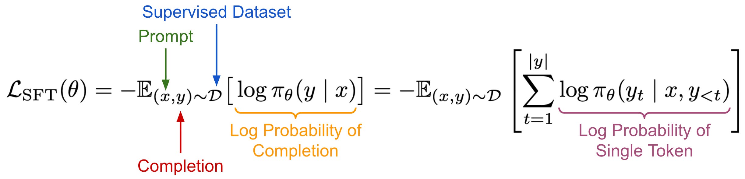
Training objectives. In SFT, we have a fixed dataset of supervised examples over which we are training our LLM. The training objective aims to minimize the model’s negative log-likelihood over this dataset, as shown below.
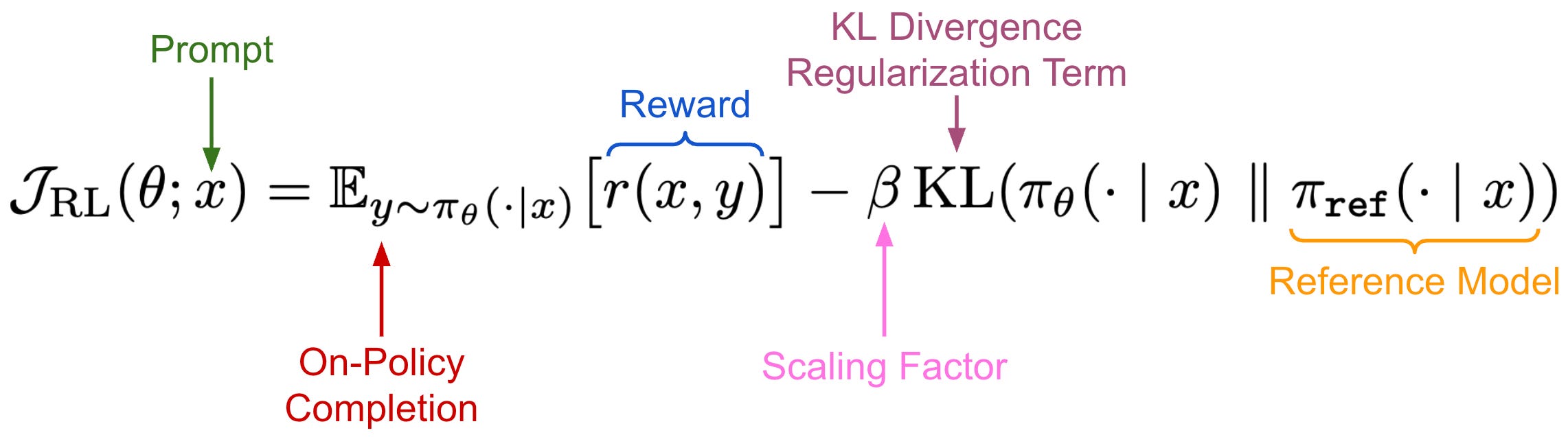
In contrast, RL uses the objective shown below, which focuses on maximizing the reward—such as a binary correctness signal in RLVR—of on-policy completions sampled for prompts taken from a fixed dataset. Optionally, we can include a KL divergence regularization term that penalizes the model for producing an output distribution that differs significantly from some reference model2.
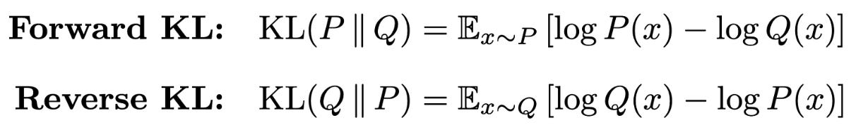
Forward and reverse KL. One possible way to view the SFT and RL training objectives is through their relation to the KL divergence. Formally, the KL divergence is a measure for the divergence between two probability distributions; see here for full details. For two probability distributions P and Q, we can define the forward and reverse KL divergences as shown in the figure below.
In the LLM domain, these probability distributions are usually the next token distributions outputted by our LLM. A key difference between the forward and reverse KL divergence lies in the sampling—the distribution from which we sample in the above expectations changes. Specifically, we are either sampling from our dataset (offline) in SFT or from the LLM itself (online or on-policy) in RL.
SFT ≈ forward KL. Using these concepts, we can show that the training objective used by SFT is equal to the forward KL divergence up to a constant. Let’s call the optimal (or target) distribution for our dataset π_*. We can show the following for the relationship between this objective and the forward KL divergence, where H(π_*) denotes the entropy3 of the optimal distribution over the SFT dataset.
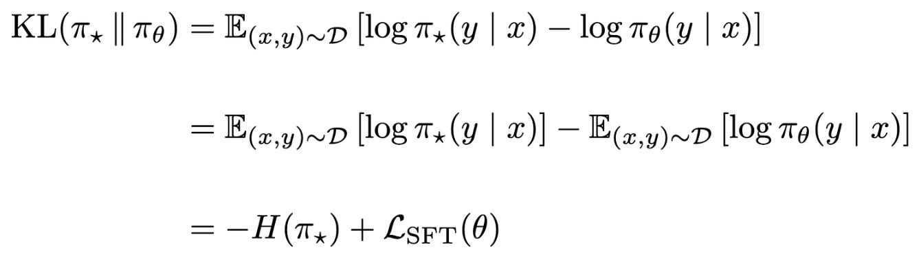
In the above expression, the entropy of the optimal distribution is a constant, so the forward KL and SFT training objective are equal up to a constant—minimizing forward KL is equivalent to minimizing the negative log-likelihood objective.
RL ≈ reverse KL. As mentioned previously, RL tries to maximize the reward of on-policy completions while minimizing KL divergence with respect to a reference policy. We can actually derive a closed-form expression for the optimal solution to the RL objective. The expression for the optimal policy is shown below, where Z(x) denotes the partition function. Notably, this optimal policy expression is also the first part of deriving the training loss for DPO!
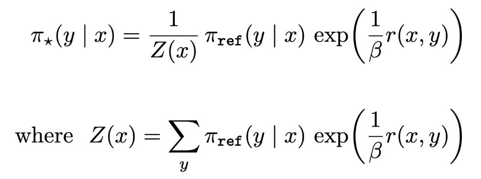
If we assume that this optimal policy π_* is our target distribution, then we can show that maximizing the RL objective is equivalent to minimizing the reverse KL divergence between this target distribution and our policy π_θ.
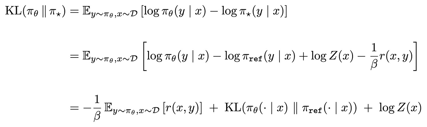
As we can see, the first line of this equation computes the reverse KL divergence relative to the KL divergence used in our derivation for the SFT objective. In the final line, we have the negative of our RL objective (plus a scaling factor of 1/β and an additional constant). Therefore, minimizing this reverse KL divergence objective would be the same as maximizing the RL training objective.
What does this tell us? Now we understand the relation of SFT and RL to the forward and reverse KL divergence, respectively. But, what do these relationships actually tell us about the objectives? SFT minimizes negative log-likelihood over a dataset, which is equivalent to minimizing the forward KL divergence. This is a mode-covering objective. Our model is heavily penalized for assigning low probability to any completion that is found in the data—the model must “spread” its probability mass across all possible completions or modes in the data.
On the other hand, RL maximizes rewards of on-policy completions, which is equivalent to a reverse KL objective and is mode-seeking. Put differently, the model prioritizes high-reward outputs, even at the cost of ignoring output modes.
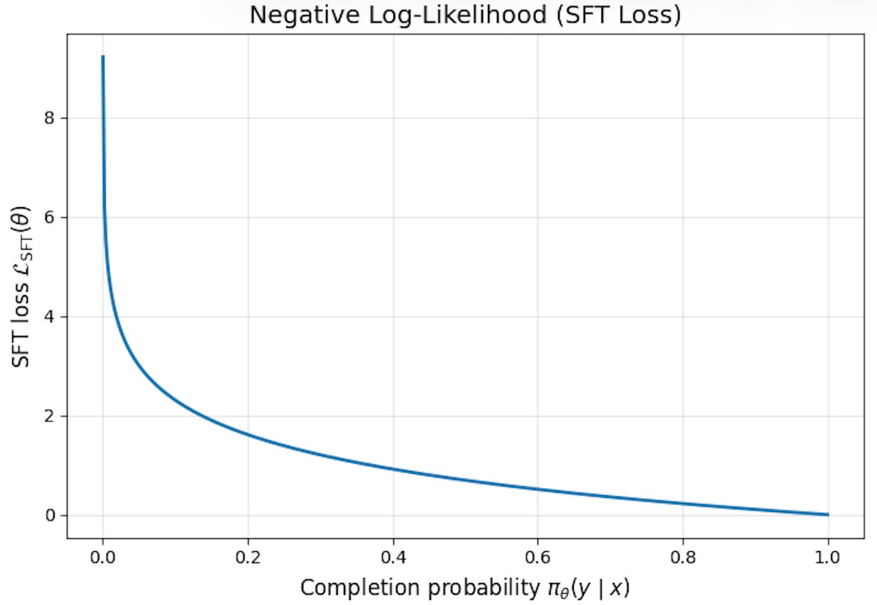
In SFT, the model’s loss increases exponentially if we assign near-zero probability to any completion in the dataset—this is due to the shape of the negative log-likelihood curve (shown above)! Such a property is not true of RL, as we are simply maximizing the reward of on-policy completions. Assigning near-zero probability to a completion will prevent this particular completion from being sampled during RL, but reward can still be maximized over the completions that are sampled. This is a fundamental property of RL that creates favorable behavior with respect to minimizing catastrophic forgetting during continual learning.
Reinforcement Finetuning Naturally Mitigates Forgetting in Continual Post-Training [1]
Continual learning can be viewed as a continued post-training process for an LLM. In this setup, the same base LLM undergoes extensive post-training over an evolving and expanding data stream, forcing the model to adapt to new requirements and learn new skills or knowledge without losing existing capabilities. However, avoiding catastrophic forgetting in this scenario is difficult. In [1], authors consider this continual post-training setup and analyze the best learning paradigm—either supervised finetuning (SFT) or reinforcement learning (RL)—for maximizing performance and minimizing forgetting.
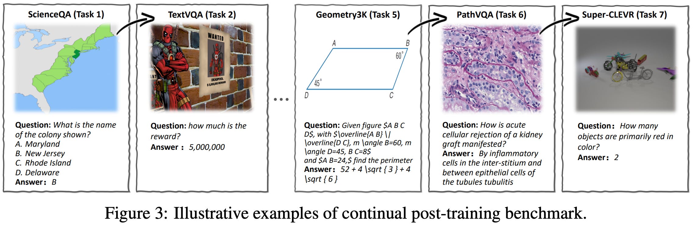
Continual post-training. In the real world, continual learning is messy—the LLM will be constantly exposed to new data from various sources—but a more organized proxy setup is needed for research. A common way to simulate continual learning is via a sequential learning (or batch-incremental) setup, where the LLM is sequentially exposed to an ordered group of datasets. In [1], authors choose seven datasets that cover a wide scope of multi-modal (vision) use cases: ScienceQA, TextVQA, VizWiz, Geometry3K, GQA, PathVQA, and Super-CLEVR.
“A higher AvgAcc indicates better overall performance, while an FM closer to zero signifies less forgetting and better knowledge preservation.” - from [1]
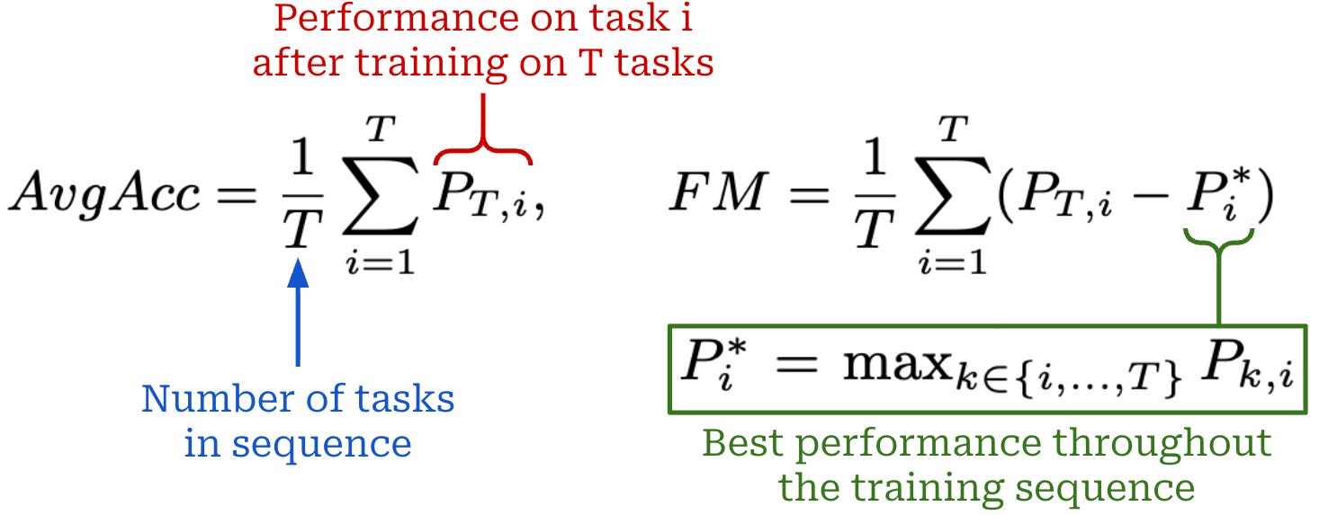
Evaluation metrics. Our goal in continual post-training is to i) maximize the LLM’s performance on each new task and ii) avoid performance degradation—or catastrophic forgetting—on prior tasks. Assume that the LLM is evaluated on all tasks after each training round, yielding performance P_{t, j} on task j after learning for task t is complete. We can then capture key performance properties of continual post-training via the following two metrics:
Average accuracy (AvgAcc): the average accuracy of the model across all tasks after training on the final task
Thas completed.Forgetting measure (FM): the average difference between the model’s final accuracy for a task and the best accuracy observed for that task throughout all
Trounds of the training sequence.
After the end of the continual post-training process, the above metrics are computed over the test sets of all previously-encountered tasks. Going further, authors in [1] also measure performance on several general LLM benchmarks (i.e., MMMU, MMLU-Pro, and POPE) at the end of the continual post-training process to check for any impact on the model’s general capabilities.
SFT versus RL. Continual post-training experiments are performed in [1] using the Qwen-2.5-VL-7B-Instruct model, which is sequentially trained on data from each of the seven benchmarks. Notably, no replay buffer or data from prior tasks is used when training on new tasks, so the model’s ability to avoid forgetting is entirely dependent upon mechanics of the learning algorithm. As mentioned before, two types of learning algorithms are used:
For RL, we derive rewards using a standard reasoning model setup that combines the verifiable reward with a format reward that encourages the model to i) wrap its reasoning trace in <think> tokens and ii) mark its output with a \boxed{} label. Models output a reasoning trace prior to their final output, though tests are performed both with and without reasoning for all training setups.
RL forgets less. The results of the continual post-training experiments in [1] are depicted below. SFT clearly leads to catastrophic forgetting of previously-learned tasks, which gets worse as tasks move further into the past—forgetting is worst on initial tasks in the sequence. More specifically, we see an average accuracy of 54% with SFT, while multi-task training on all tasks reaches an average accuracy of 62.9%. Similarly, a FM of -10.4% is also observed for SFT, indicating that most tasks degrade noticeably in performance throughout continual post-training.
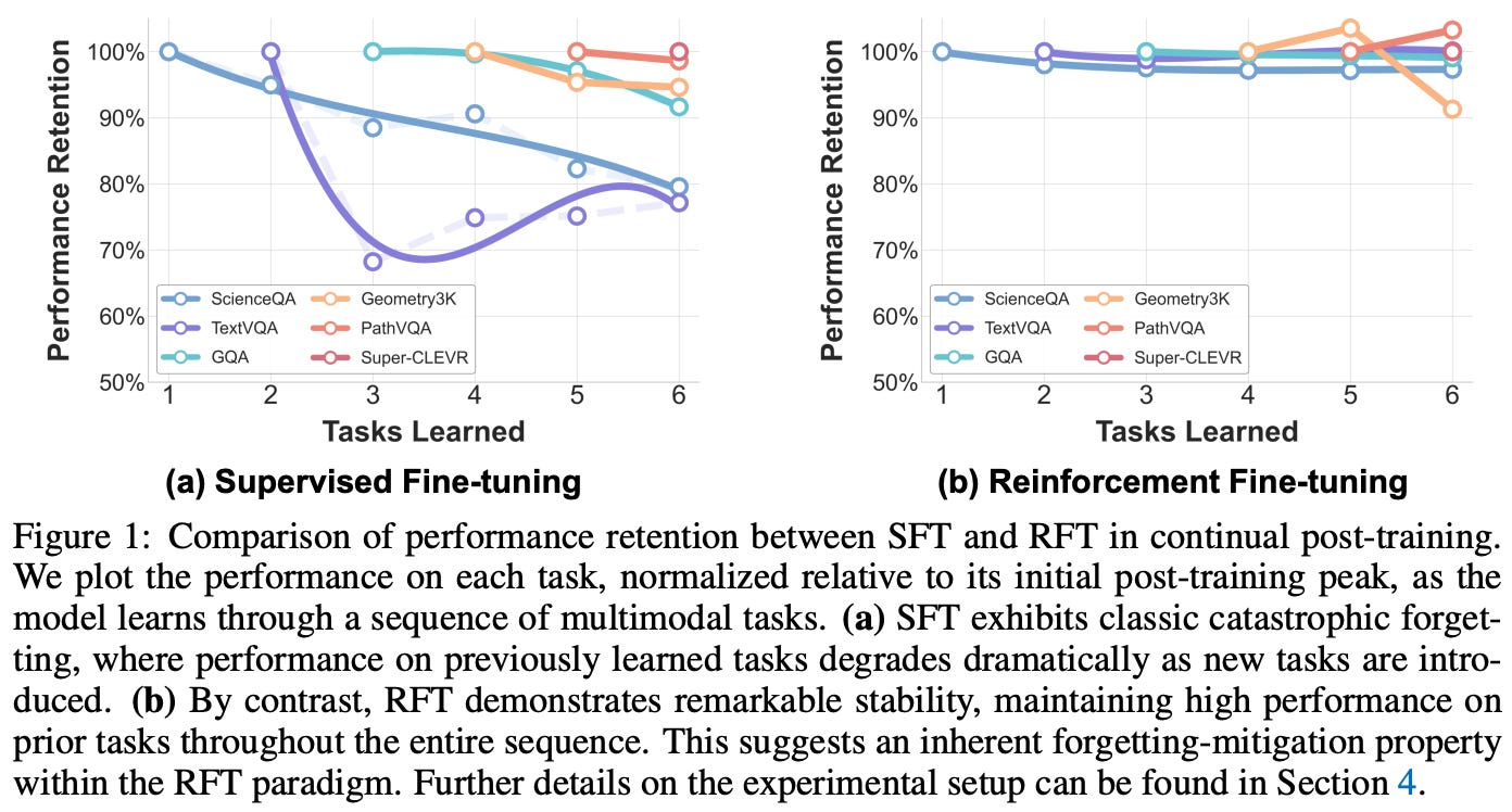
While SFT struggles to mitigate forgetting, RL naturally adapts well to new tasks. For GRPO, we observe an average accuracy of 60% (i.e., slightly below multi-task learning) and an FM of -2.3%. Additionally, the final accuracy on ScienceQA—the first task in the sequence—is 93%, compared to a peak accuracy of 95.6%. These results show that RL strikes a strong balance between learning and remembering.
“Without any data replay, continual post-training with RFT can achieve comparable performance with that of multi-task training, which is not achievable even when equipping SFT with continual learning strategies.” - from [1]
Influence on general capabilities. In the same vein, SFT-based continual post-training also degrades general model capabilities; see below. In contrast, we see in [1] that RL maintains—or even slightly enhances—performance on general benchmarks. For example, models sequentially trained with GRPO improve from an initial accuracy of 52.1% to a final accuracy of 54.2% on MMMU!
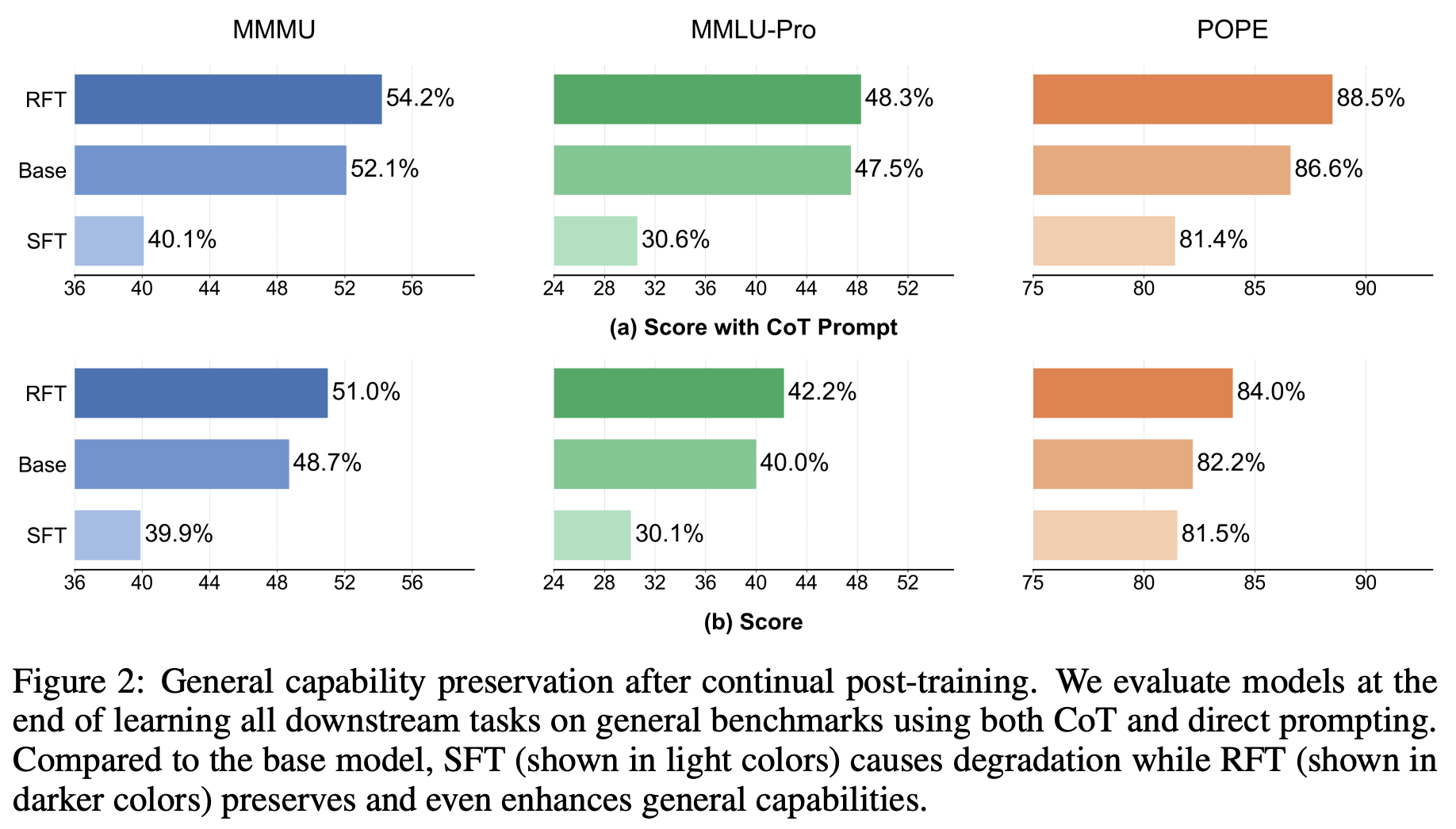
Such an ability to maintain performance on general benchmarks is a desirable aspect of continual learning. Ideally, we want the LLM to adapt to new tasks while maintaining its existing, foundational capabilities as much as possible.
Why does RL forget less? Given the above results, we might begin to wonder: Why does RL have the ability to naturally avoid catastrophic forgetting? Of course, it is possible that such continual learning abilities are directly attributable to RL itself. However, authors in [1] also consider two alternative explanations for the lack of catastrophic forgetting:
The use of a KL divergence term in RL regularizes the training process and acts as a form of knowledge distillation that preserves prior knowledge.
The use of long CoT reasoning in models trained with RL leads to a more robust knowledge base that is better protected from forgetting.
To test whether these factors help with avoiding catastrophic forgetting, three setups are tested that ablate the use of KL divergence and long CoT reasoning. Interestingly, we learn from testing these setups that removing KL divergence, despite degrading the stability of RL training4, does not lead to any degradation in performance metrics for continual post-training. Additionally, models that do not output a reasoning trace resist catastrophic forgetting similarly to those that do. Using CoT reasoning improves baseline model performance, but continually trained models in either setup see the same amount of catastrophic forgetting.
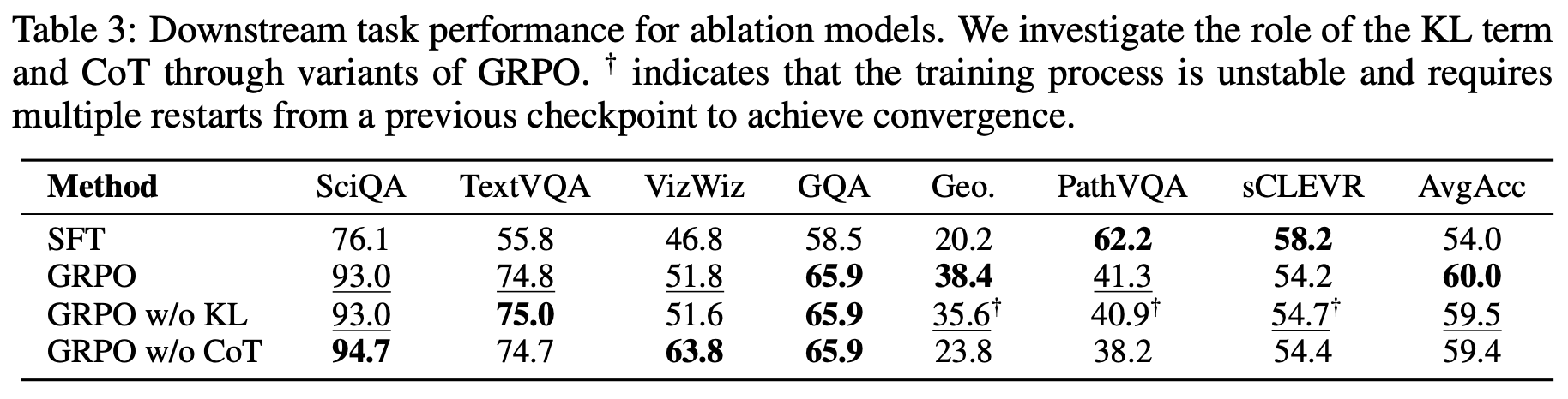
The results of these ablation experiments are outlined in the table above. The impressive performance of RL in continual post-training experiments does not seem to stem from the use of KL divergence or long CoT reasoning. Rather, the ability to perform continual learning seems to be an inherent property of RL training. Insight as to how RL avoids forgetting is provided by theory in [1] showing that RL naturally scales policy updates according to the variance of the reward signal, leading to more conservative updates for important or sensitive parameters.
“We offer a theoretical perspective suggesting that RFT’s updates are inherently more conservative in parameter subspaces sensitive to prior tasks. This conservatism is naturally scaled by the variance of the reward signal, creating a data-dependent regularization that dampens updates on uncertain samples, thus protecting established knowledge.” - from [1]
Retaining by Doing: The Role of On-Policy Data in Mitigating Forgetting [2]
Work in [2] shares a very similar focus to the paper above—trying to compare SFT and RL in the context of continual learning. However, a different experimental setup is used that considers three domains: instruction following (IFEval), general skills (MMLU), and arithmetic reasoning (Countdown). Beyond these target tasks that are used for training and evaluation, a few non-target tasks (i.e., MATH and two safety benchmarks) are included to provide a wider evaluation suite. We do not train the LLM over a sequence of tasks in [2]. Rather, the LLM is trained over one target task—a domain adaptation setup—and we measure performance via:
The accuracy gain on that target task.
The average accuracy drop across all non-target tasks.
Notably, the lack of multi-step sequential learning makes this setup less realistic. In [1], we see that the impact of catastrophic forgetting is greater after several training rounds. However, the domain adaptation setup in [2] does allow us to efficiently analyze the forgetting mechanics of different learning algorithms. The following learning algorithms are considered in [2]:
SFT training on responses from a teacher model (Llama-3.3-70B-Instruct).
Self-SFT training, which performs SFT-style training over responses from the initial policy (before training) or reference model.
RL training using GRPO with verifiable rewards—a standard RLVR setup.
Both SFT variants filter completions based on correctness, as determined by deterministic verifiers for each domain. Self-SFT is a rejection sampling setup (i.e., incorrect responses are rejected) that is used as a simple baseline, whereas the SFT setup performs offline knowledge distillation from a larger model. Self-SFT is an offline approach as well because completions are sampled from the initial model, rather than on-policy. The same verifiable correctness signal used for filtering completions in SFT variants is also used as the reward signal in RL.
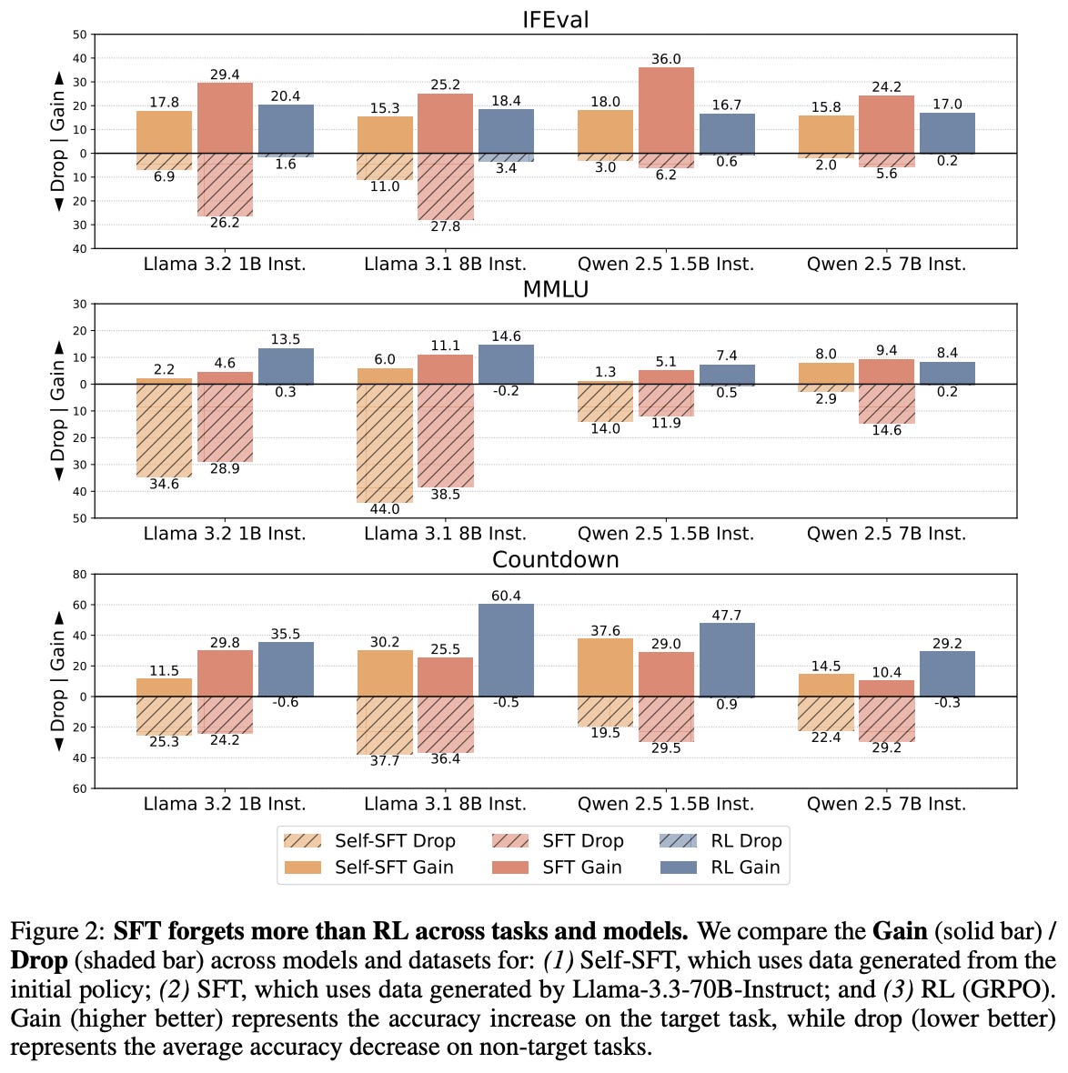
RL forgets less (again). Experiments are performed in [2] using Qwen-2.5 and Llama-3 models with up to 8B parameters. As shown above, higher levels of forgetting—as measured via the average accuracy drop across non-target tasks—are observed with SFT compared to RL. In fact, Qwen-2.5 models see <1% average accuracy drop across all tasks and model scales for RL training, whereas the average accuracy drop with SFT reaches nearly 30% in some cases.
“RL leads to less forgetting than SFT while achieving comparable or higher target task performance… SFT suffers from severe forgetting, whereas RL can achieve high target task performance without substantial forgetting.” - from [2]
Despite the ability of RL to avoid catastrophic forgetting, the results with SFT are not actually bad—there is just a clear domain tradeoff. We can achieve performance improvements in the target domain via RL training, but models trained via SFT actually perform better. Unfortunately, the superior performance of SFT in the target domain comes at the cost of degraded performance on non-target tasks. For this reason, the comparison is not as simple as RL > SFT. Rather, RL and SFT lie at different points on the Pareto frontier of target and non-target task accuracy—better performance in one domain comes at the expense of the other.
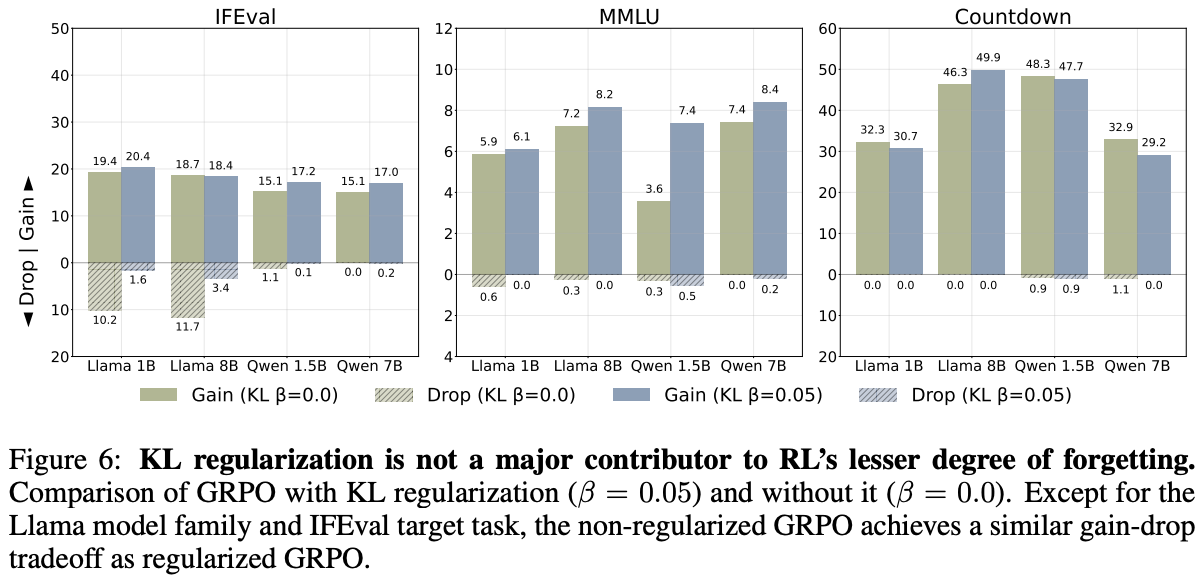
Benefits of on-policy data. Similar to work in [1], authors in [2] show the lack of catastrophic forgetting in RL is not due to the inclusion of a KL divergence term in the objective; see above. Interestingly, the exact advantage formulation used by GRPO is also found to have little impact on continual learning capabilities—a naive REINFORCE-based RL setup is shown to mitigate forgetting to a similar extent. It is possible, however, that the continual learning abilities of RL stem from its use of on-policy samples—unlike the offline dataset used by SFT—during training. To test this theory, we consider the following training setups:
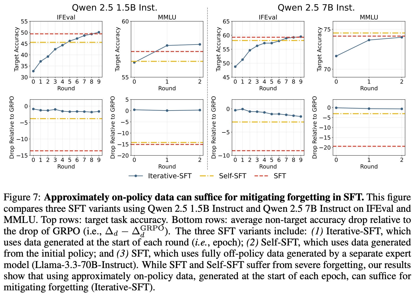
On-policy SFT: running SFT using fully on-policy samples that are directly obtained from the RL training process.
Iterative SFT: re-generating data for SFT after every epoch using the current policy (i.e., a partially on-policy approach).
Put simply, these approaches adapt SFT to use on-policy data, which allows us to decouple the impact of RL training and on-policy data. The use of iterative SFT also allows us to test a semi-on-policy scenario, which samples fresh on-policy data at the end of each epoch (i.e., instead of generating new samples during each training iteration). This coarse-grained approach to on-policy data has efficiency benefits—we can adjust the regularity with which we sample fresh on-policy data.
“We find that for SFT, while generating data only from the initial policy is not enough, approximately on-policy data generated at the start of each epoch can suffice for substantially reducing forgetting. This suggests a practical guideline for LM post-training: leveraging on-policy data, potentially sampled asynchronously or at the start of each epoch for improved efficiency, can reduce unintended disruption of the model’s existing capabilities.” - from [2]
Experiments with these training algorithms provide empirical evidence that on-policy data is a key contributor to the success of RL in the continual learning domain. Specifically, models trained via on-policy SFT mitigate forgetting to a similar extent as those trained via RL. Additionally, the data used does not need to be fully on-policy—similar trends are observed with iterative SFT; see below.
Mode-seeking versus mode-covering. Intuitively, we might assume that the mode-covering nature of SFT would allow the model to maintain probability mass across all tasks and, therefore, avoid catastrophic forgetting. As we have seen, however, the opposite is true in practice. Such a finding is due to the fact that we are only training our model over a small subset of the model’s total data distribution in most of these experiments. Potentially our observations would be different if we were able to retain the LLM’s entire training dataset within a replay buffer, but implementing such an approach efficiently would be incredibly difficult.
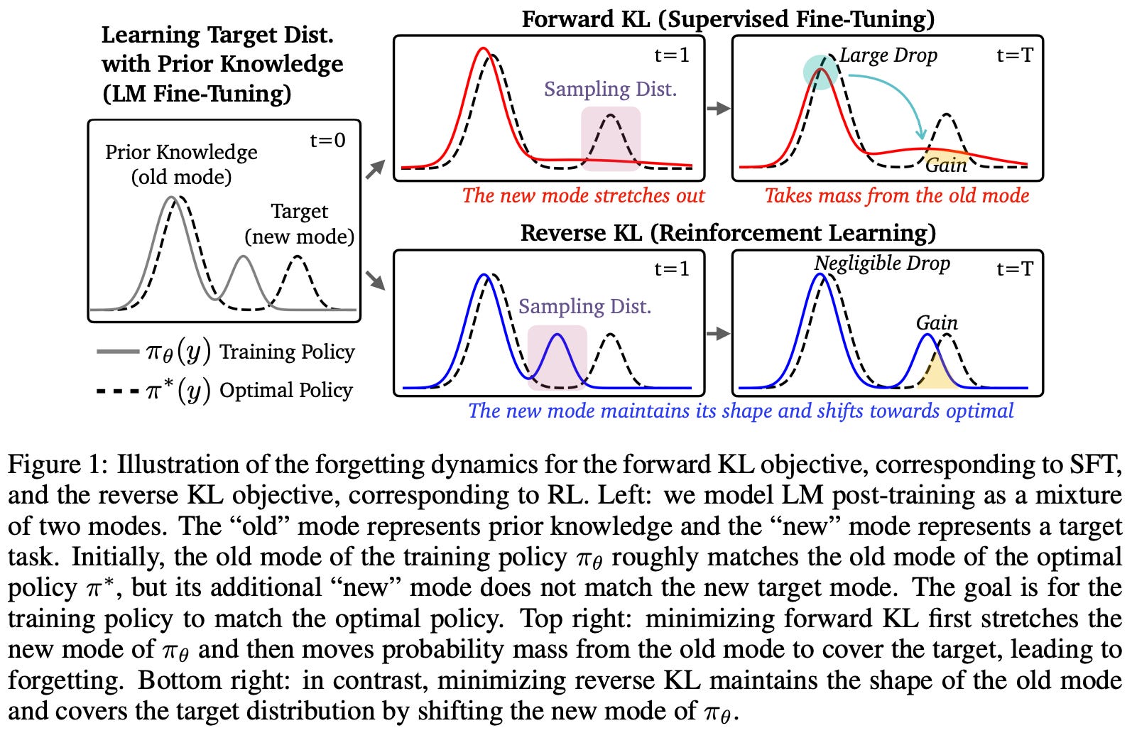
In the standard LLM post-training setup, the mode-seeking behavior of RL is more robust to catastrophic forgetting. To explain this phenomenon, authors in [2] construct a simplified setting shown above, which illustrates the dependence of forgetting on the modality of the underlying target distribution. If our target distribution is multi-modal, which is likely to be true for an LLM, then the mode-seeking nature of RL actually leads to less forgetting relative to a mode-covering objective like SFT. The simplified distribution that is constructed in [2] has two modalities corresponding to old and new knowledge. For such a distribution, the forward KL objective yields noticeable forgetting while minimizing the reverse KL allows both modes of the target distribution to be properly captured.
RL’s Razor: Why Online RL Forgets Less [3]
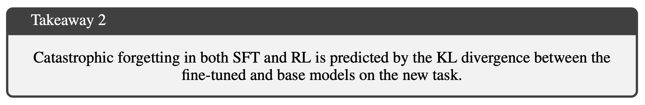
As we know, SFT and RL achieve comparable performance when training on a new task but have drastically different forgetting dynamics. In most cases, gains on new tasks with SFT come at the cost of erasing prior knowledge, while RL is much better at protecting old capabilities; see below. By studying this gap in performance, authors in [3] identify a metric that reliably predicts the amount of forgetting that occurs for both SFT and RL: the distributional shift—measured via KL divergence—between the base and finetuned models on the target task.
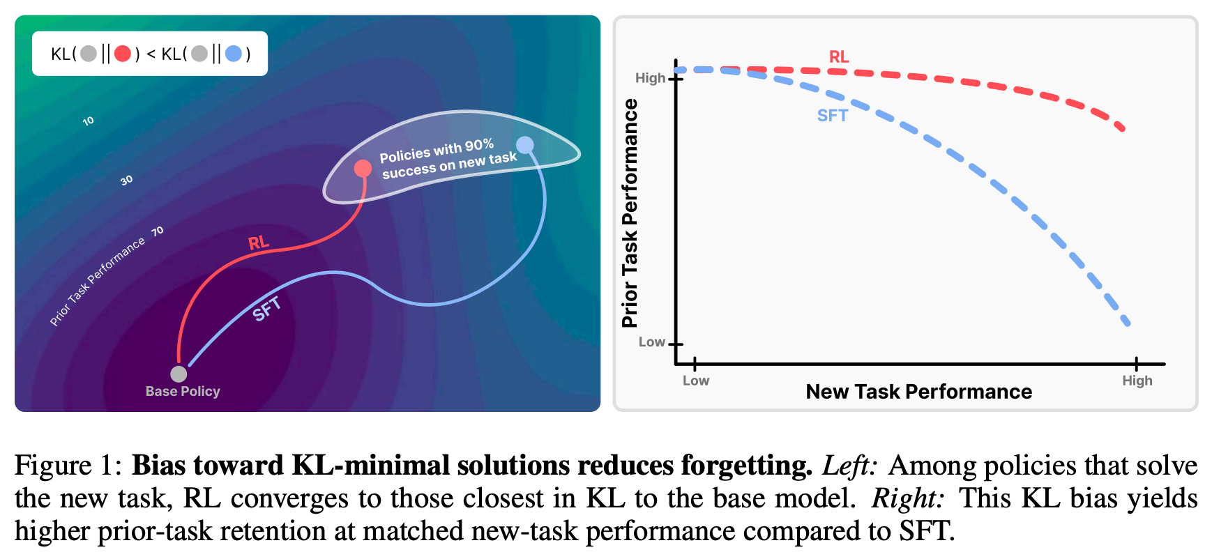
RL’s Razor. In addition to discovering this relationship between the underlying distribution shift and forgetting, we see in [3] that the finetuned models from SFT and RL have unique properties:
RL is biased towards solutions that minimize distributional shift.
SFT can converge to solutions arbitrarily far away from the base model.
Such a property naturally implies the improved continual learning abilities of RL. By discovering a solution that minimizes distributional shift, we also minimize the amount of forgetting that occurs; see above. The bias of RL towards nearby solutions that minimize catastrophic forgetting is referred to in [3] as “RL’s Razor”5.
“RL’s Razor: among the many high-reward solutions for a new task, on-policy methods such as RL are inherently biased toward solutions that remain closer to the original policy in KL divergence… the KL divergence between the fine-tuned model and the base model, measured on the new task, reliably predicts… forgetting.” - from [3]
Distribution shift. In the LLM domain, we often measure the KL divergence between the next token distributions of two models. For example, the RL training objective has a KL divergence term that regularizes drift between the current and reference policy, where the KL divergence is computed using on-policy samples taken from the current policy during RL training. In [3], authors compute the KL divergence over data from the task on which our policy is being finetuned (i.e., the target task). We are restricted to using the target data because we rarely have access to the pretraining data (or any prior tasks) on which an LLM was trained.
This KL divergence between base and finetuned models on the target dataset can be viewed as capturing the distributional shift from training. We are computing the divergence between models before and after training over the training data itself. When measured in this way, the distributional shift is found to be consistently predictive of the amount of forgetting that occurs. Given that no prior data is used to compute this KL divergence, such a finding is highly non-trivial!
Experiments in [3] are performed using both vanilla SFT and RL with GRPO. The RL setup uses standard verifiable rewards and no KL divergence regularization. Similarly to [2], the base model (Qwen-2.5-3B-Instruct) is trained on one target task (i.e., Open-Reasoner-Zero, ToolAlpaca, or the Chemistry L-3 subset of SciKnowEval) and evaluated on both the target task and set of prior tasks (i.e., HellaSwag, TruthfulQA, MMLU, IFEval, WinoGrande, and HumanEval). Given that hyperparameter settings can massively impact results in a continual learning setup6, a wide variety of hyperparameters are tested for each task and results are visualized as a Pareto frontier constructed by all possible settings.
Lower KL leads to less forgetting. RL training improves target task performance while keeping performance on prior tasks stable. However, improvements in performance obtained via SFT come at the cost of noticeable forgetting. The deterioration in performance is most visible in the math domain; see below.
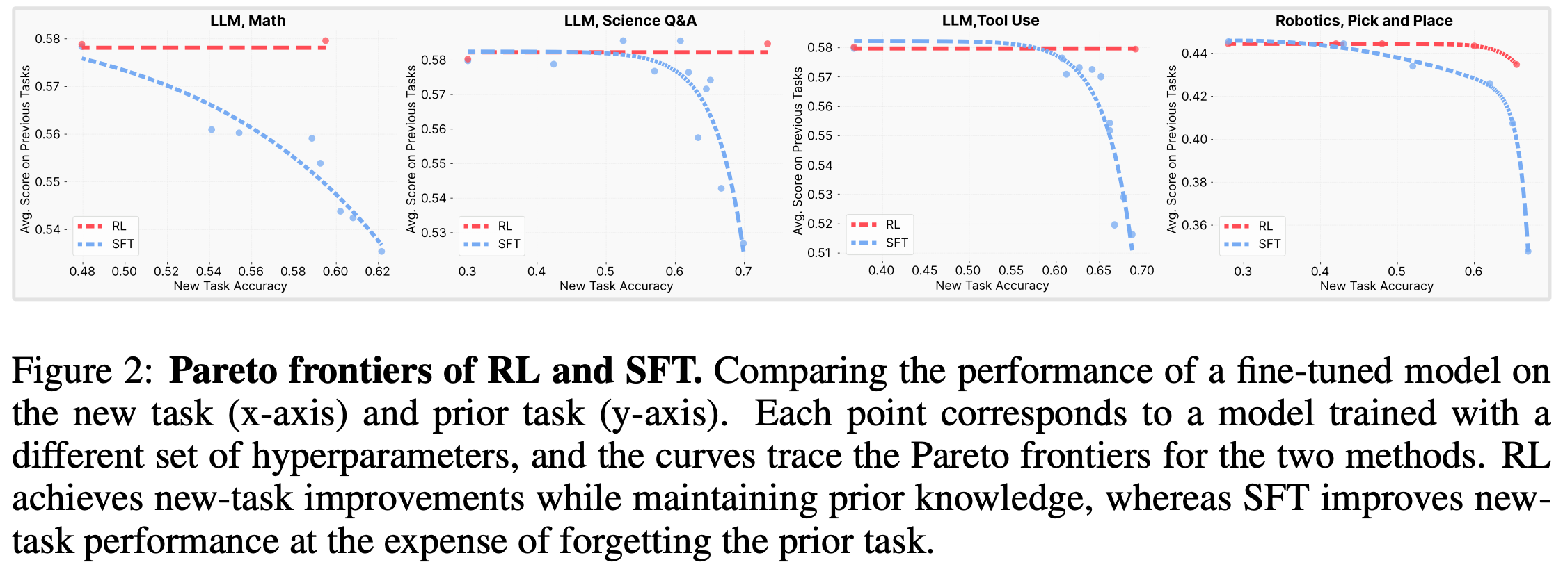
Identifying the cause of such forgetting is difficult due to the high computational cost of RL training—testing each hypothesis is quite expensive! To make this search more tractable, a toy setting is created based on the MNIST and FashionMNIST datasets for which RL training is much faster. Using this setting, a variety of candidate metrics are tested for a relationship to catastrophic forgetting:
The magnitude of changes to model parameters.
The sparsity of weight updates.
The rank of policy gradients throughout training.
The only quantity that demonstrates a consistent relationship with the amount of catastrophic forgetting is the KL divergence between base and finetuned models over the target dataset; see below. The fact that the rank or sparsity of policy gradient updates is unrelated to forgetting is notable, as prior research [4] has shown that RL works surprisingly well even when using LoRA with a low rank. Such a finding indicates that the updates being produced by RL are potentially sparse or low rank, which could help to reduce forgetting. However, we see in [3] that the story is not this simple. Rather, the benefits of RL stem from an implicit KL regularization—or RL’s Razor—that minimizes distribution shift in training.
To further validate the relationship between the KL divergence and forgetting, authors create an “oracle” SFT distribution in their toy setting. Put simply, this experiment performs SFT on a dataset that has been analytically constructed to minimize the KL divergence between the base and finetuned models. As shown above, running SFT on this data yields an even better tradeoff than RL—the model performs better on the target task without sacrificing prior task performance.
“RL performs well because its on-policy updates bias the solution toward low-KL regions, but when SFT is explicitly guided to the KL-minimal distribution, it can surpass RL.” - from [3]
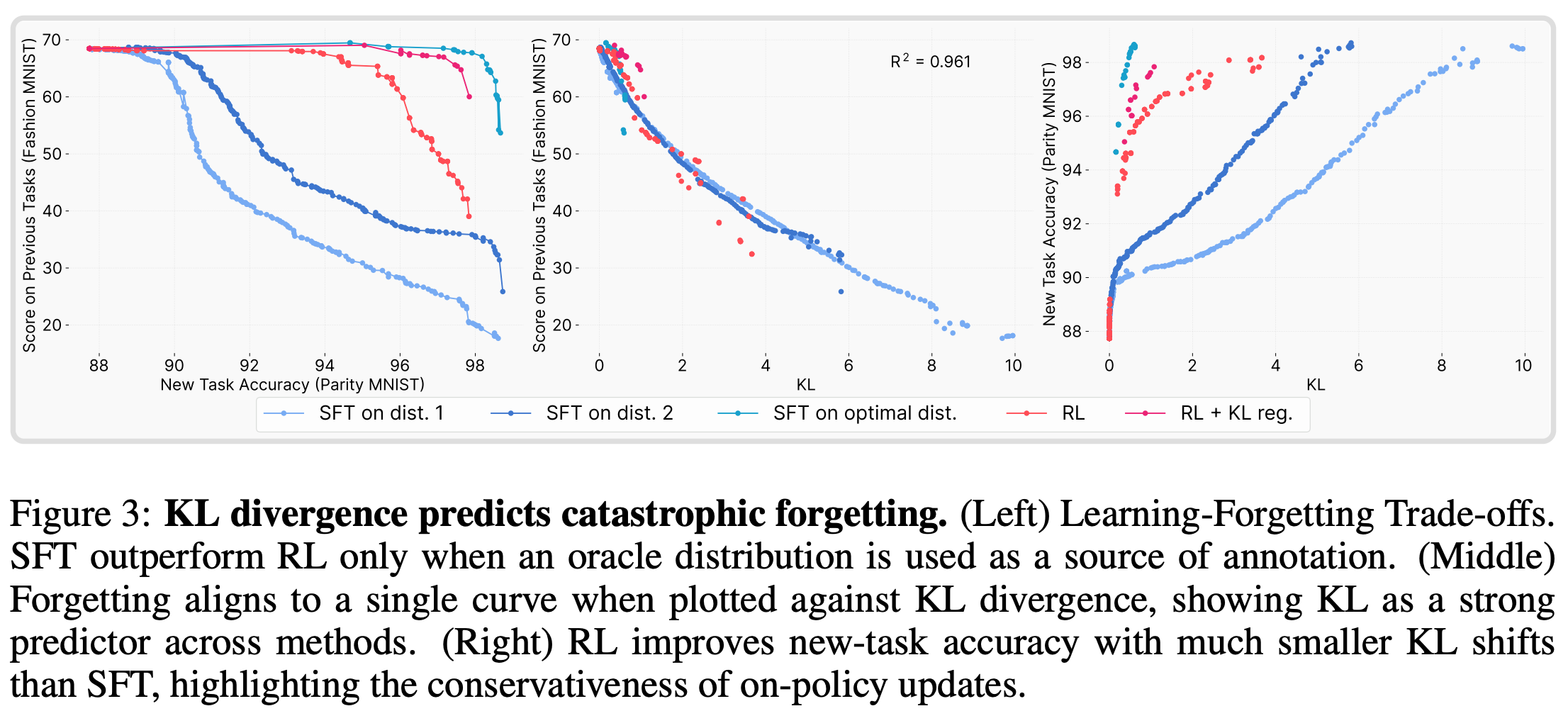
On-policy data. Beyond the toy example explained above, authors in [3] also run SFT training over on-policy data obtained during RL. The accuracy-forgetting tradeoff achieved by the resulting model matches that of those trained via RL, which aligns with prior work [2] and provides further evidence that on-policy data plays a key role in mitigating forgetting for RL. To better understand the impact of on-policy data, three different learning algorithms are tested (shown below):
Standard GRPO.
Standard SFT.
1-0 REINFORCE: an on-policy RL algorithm with a very simple advantage function (i.e., 1 if the answer is correct and zero otherwise).
SimPO [5]: an offline preference tuning algorithm that simplifies DPO by directly using the log probability of a sequence as the implicit reward and, therefore, removing the need for a reference model.
As we can see in the left half of the above figure, these experiments ablate the use of negative examples and on-policy data within the training setup. Interestingly, the 0-1 REINFORCE algorithm performs similarly to GRPO, while results with SimPO resemble those of SFT. Such results indicate that the use of on-policy data is the key contributor to RL’s lack of forgetting. We also see above that the use of on-policy data leads to minimal KL divergence between the base and finetuned models over the target distribution. Such results indicate that the implicit bias of RL towards low KL solutions stems from the online nature of training. This empirical observation is also justified by further theoretical analysis in [3].
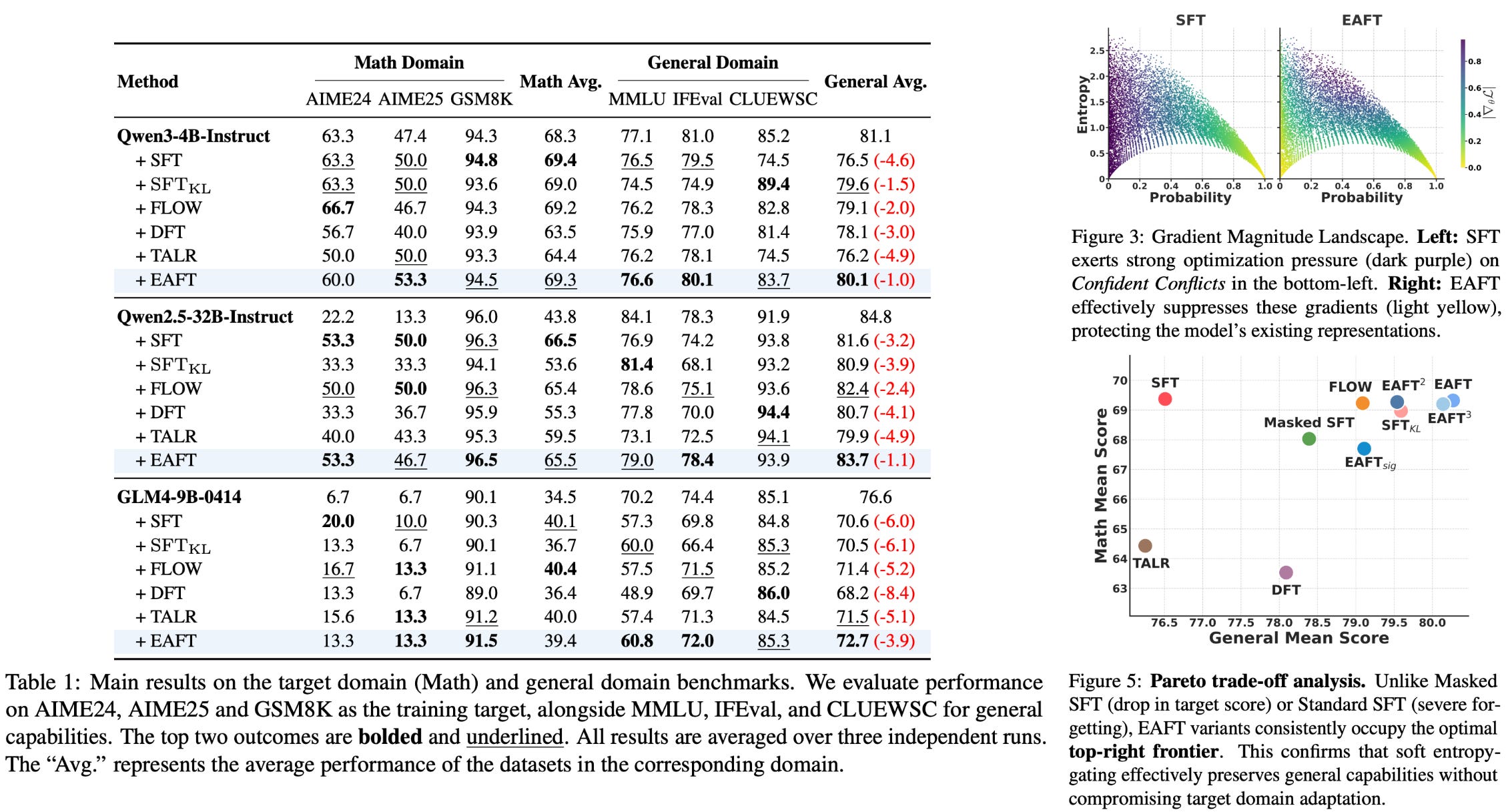
Entropy-Adaptive Fine-Tuning: Resolving Confident Conflicts to Mitigate Forgetting [6]
“While RL aligns with the model’s internal belief, SFT forces the model to fit external supervision. This mismatch often manifests as Confident Conflicts—tokens characterized by low probability but low entropy.” - from [6]
We have learned that RL avoids catastrophic forgetting much better than SFT due to its use of on-policy data, which allows for the discovery of a solution with minimal KL divergence between base and finetuned models on the target data. Although we know that these factors lead to less forgetting, we do not yet understand why this is the case. In [6], authors offer a new perspective on the forgetting properties of SFT and RL by analyzing token probabilities and entropy of models trained with these two approaches. When these two quantities are measured throughout the training process, we see that a clear gap exists:
On-policy RL tends to cluster in regions of highly-confident and correct predictions—characterized by high probability and low entropy—or exploratory completions—characterized by high entropy.
SFT has a significant cluster of tokens with both low entropy and low probability—these are referred to as “Confident Conflicts”.
To discover this distribution mismatch, token probability and predictive entropy is measured over both the SFT dataset and model-generated rollouts. This trend is visualized below, where we see that SFT data has a noticeable cluster of confident conflict tokens that does not exist when using on-policy data.
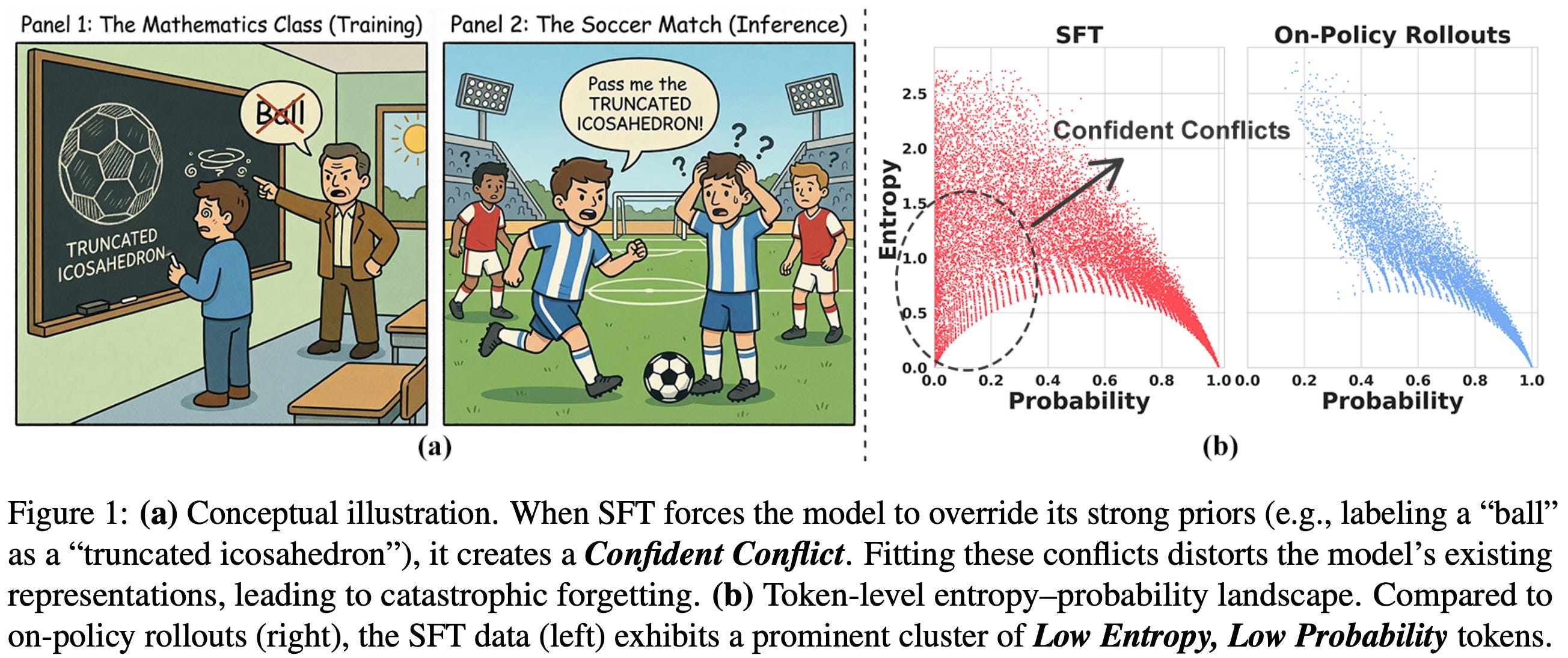
Why does this occur? We are using external supervision in SFT (i.e., an offline supervised dataset), whereas RL learns from on-policy or self-generated data. In some cases, training the model on external data forces it to mimic outputs that align poorly with its current next distribution—confident conflicts occur when external data has a strong conflict with the model’s prior. As a result, gradient updates can become large and destructive, leading to catastrophic forgetting.
“Because the model strongly favors another token, fitting the target requires substantial parameter updates, which can overwrite general representations in the base model. By contrast, when the model is uncertain (high entropy), the gradients are smaller and updates are gentler, helping preserve the model’s original capabilities.” - from [6]
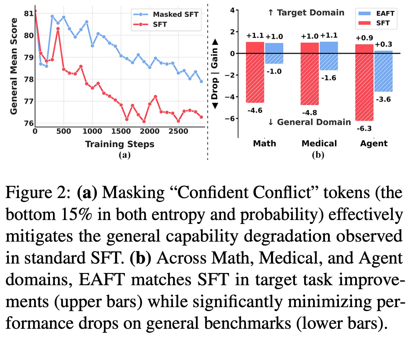
Masking conflicts. To determine whether confident conflict tokens truly lead to forgetting, authors in [6] test simply masking the loss from such tokens during SFT. Interestingly, catastrophic forgetting is significantly reduced when these tokens are masked from the training loss, indicating that confident conflict tokens play a significant role in the tendency of SFT to damage prior knowledge; see below.
Extending this idea, a novel training algorithm, called Entropy Adaptive Finetuning (EAFT), is proposed in [6] that scales the token-level cross-entropy loss by a dynamic entropy factor. The new loss formulation is outlined below, which multiplies the supervised loss by the token’s normalized entropy7. By using this token-level entropy scaling factor, we can effectively mask the loss of low entropy tokens that lead to destructive gradient updates while maintaining the full update for high entropy tokens that are beneficial for exploration.
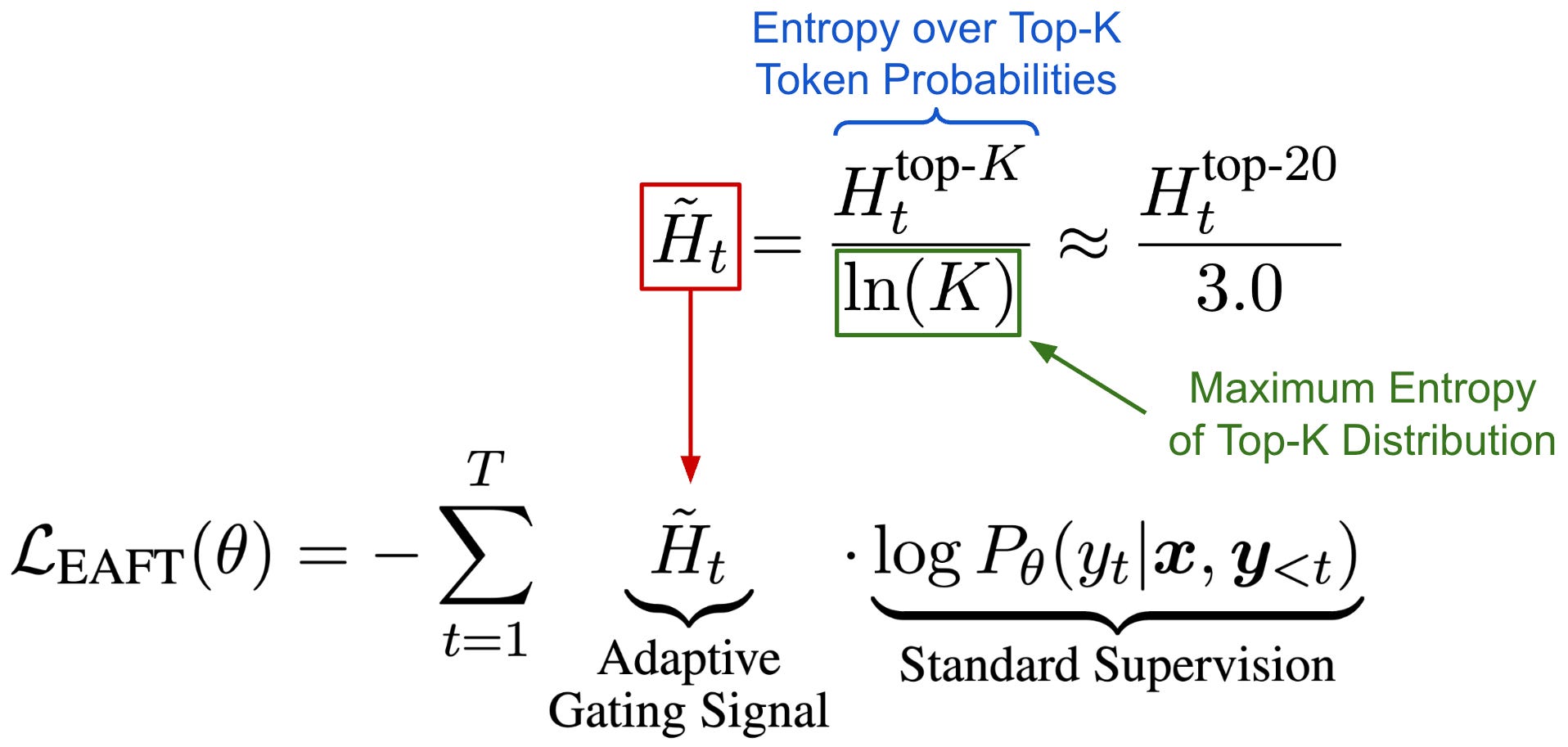
“EAFT employs a soft gating mechanism that dynamically modulates the training loss based on token-level entropy.” - from [6]
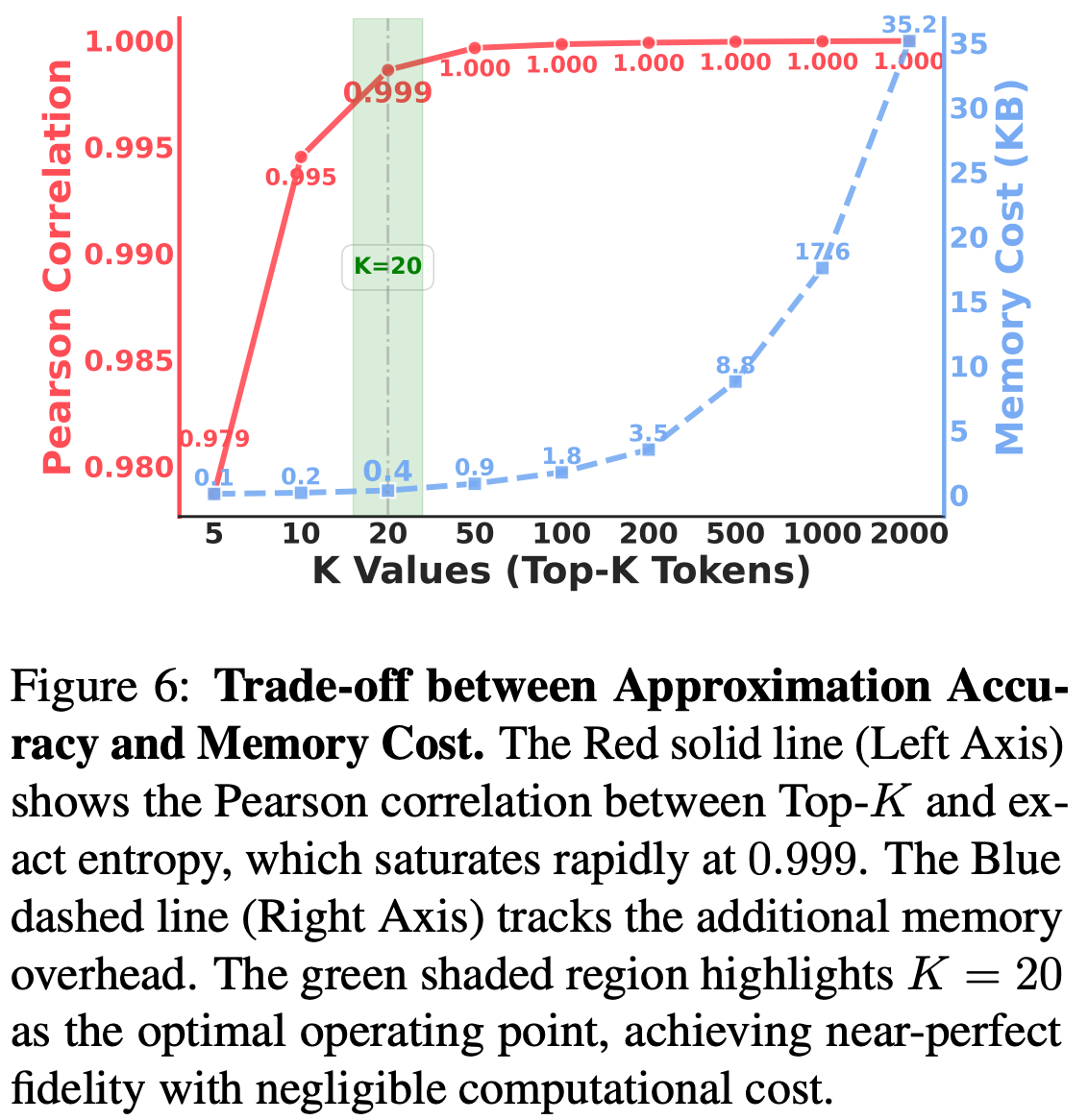
To improve the efficiency of EAFT, authors in [6] only compute entropy over the Top-K (where K = 20) tokens in the distribution. As shown in the figure below, this setting balances the tradeoff between compute and memory overhead and ensures that added computational overhead relative to vanilla SFT is minimal.
Results on Math. EAFT is validated in the Math domain using models across multiple families ranging from 4B to 32B parameters. Training prompts are sourced from NuminaMath, BigMathVerified, and Nemotron-CrossThink, while completions are sampled from Qwen-3-235B-A22B-Instruct. Both in-domain and general benchmarks are used for evaluation. Models trained with EAFT perform well in the target domain while maintaining performance on general benchmarks; see below. Additionally, EAFT is found to effectively filter confident conflict samples during the training process, as demonstrated by the visible reduction in gradient magnitude within the confident conflict zone of the below figure. These results are further validated in experiments in the medical and tool use domains.
Does RL Generalize Well?
So far, we have focused on retaining old skills while learning new ones. A closely related question is whether the same mechanisms that reduce forgetting also improve transfer and out-of-distribution generalization. The fact that RL performs well in a continual learning setting has important implications for its generalization properties. Put simply, RL training tends to benefit more than just the target domain. As we will see in the next few papers, there are many examples of RL training yielding cross-domain performance benefits or improving the generalization of an LLM to some other task. Much of this analysis is similar in nature to what we have seen for continual learning, but the emphasis shifts from remembering prior tasks to generalizing beyond the training distribution.
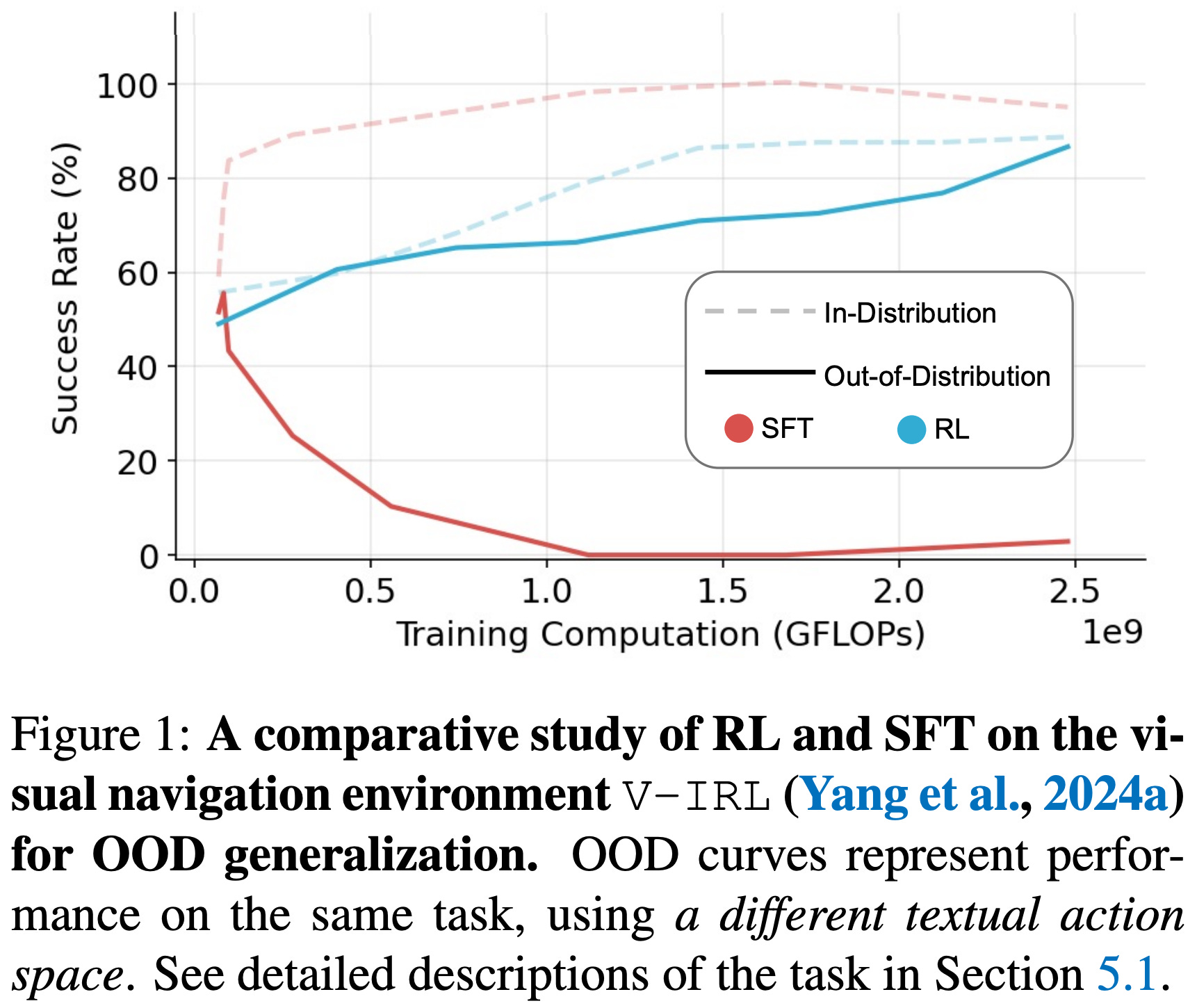
SFT Memorizes, RL Generalizes [7] performs a comparative post-training analysis between SFT and RL on both language-only and vision-language tasks. The main results of this analysis are depicted above, where we see that:
Both SFT and RL improve in-domain performance.
Only RL generalizes well to new tasks or data.
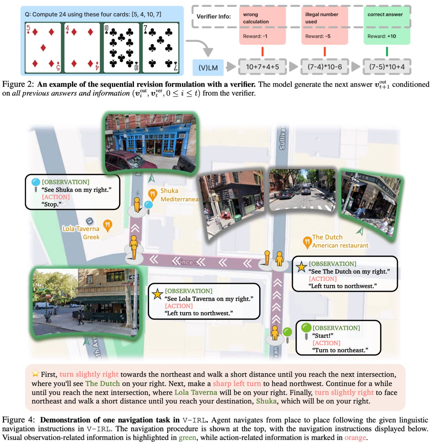
Experiments in [7] use Llama-3.2-Vision-11B as the base model and train over two synthetic tasks (shown below) that test distinct forms of generalization:
GeneralPoints: A card game that requires the model to create equations to reach a target number using four given cards. We can test rule-based generalization by changing the mapping of face cards to numbers.
V-IRL: A navigation task that has the model reach a destination using visual landmarks and spatial reasoning. We can test generalization by varying the available action space or visual context.
Each task can be setup as both a language-only and vision-language problem. In all experiments, RL tends to promote out-of-distribution generalization while SFT actually damages it. For example, the out-of-distribution performance of models trained with RL improves by 3.5% and 11.0% on language-only GP and V-IRL. For vision-language variants, this performance improvement is slightly less pronounced (i.e., 3.0% and 9.3% on GP and V-IRL) but still present. In stark contrast, SFT degrades out-of-distribution performance by as much as 79.5%.
As an interesting side note, authors in [7] also find that RL benefits the model’s underlying perception capabilities. Namely, the model actually improves in its ability to identify key vision features during training, indicating that RL is not just learning reasoning patterns but also improving fundamental abilities (i.e., perception).
“Analysis of the GP-VL task showed that RL improved the model's ability to correctly identify card values from images, suggesting that outcome-based rewards can refine perceptual processing beyond what supervised training achieves.” - from [7]
From Atomic to Composite [8] tests the generalization impact of RL training on problems that require complementary reasoning—the ability to integrate external context with the model’s parametric knowledge. To test this style of reasoning, a controlled synthetic dataset is created; see below. The dataset is based on a knowledge graph of human biographies with fixed relationships. Using this graph, we can construct multi-hop questions that test complementary reasoning by design. More specifically, questions are specifically constructed to test three levels of reasoning with increasing complexity (depicted below):
IID reasoning applies known patterns to new entities.
Compositional reasoning applies known relationships to new relational paths.
Zero-shot reasoning requires generalizing to unseen relations.
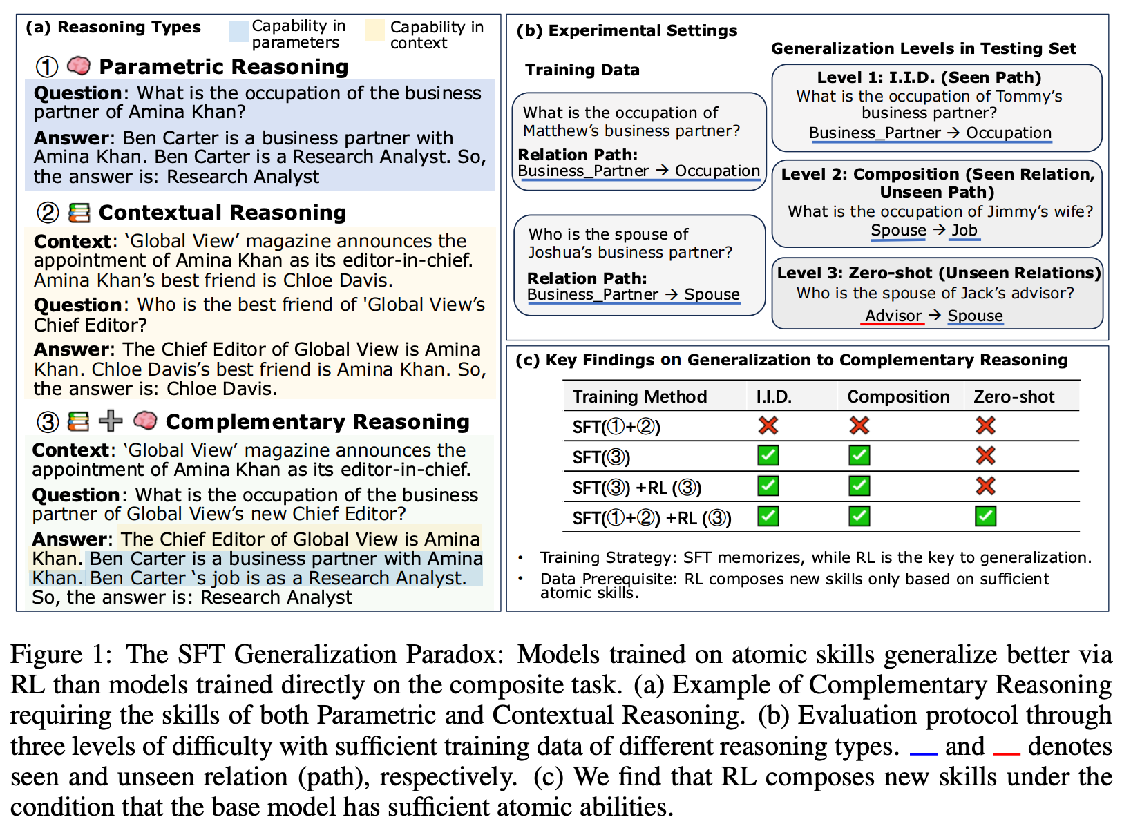
The training process in [8] starts with Qwen-2.5-1.5B, performs an initial SFT stage, then tests several combinations of SFT and RL (using GRPO with binary verifiable rewards) training. The main results of these experiments are below.
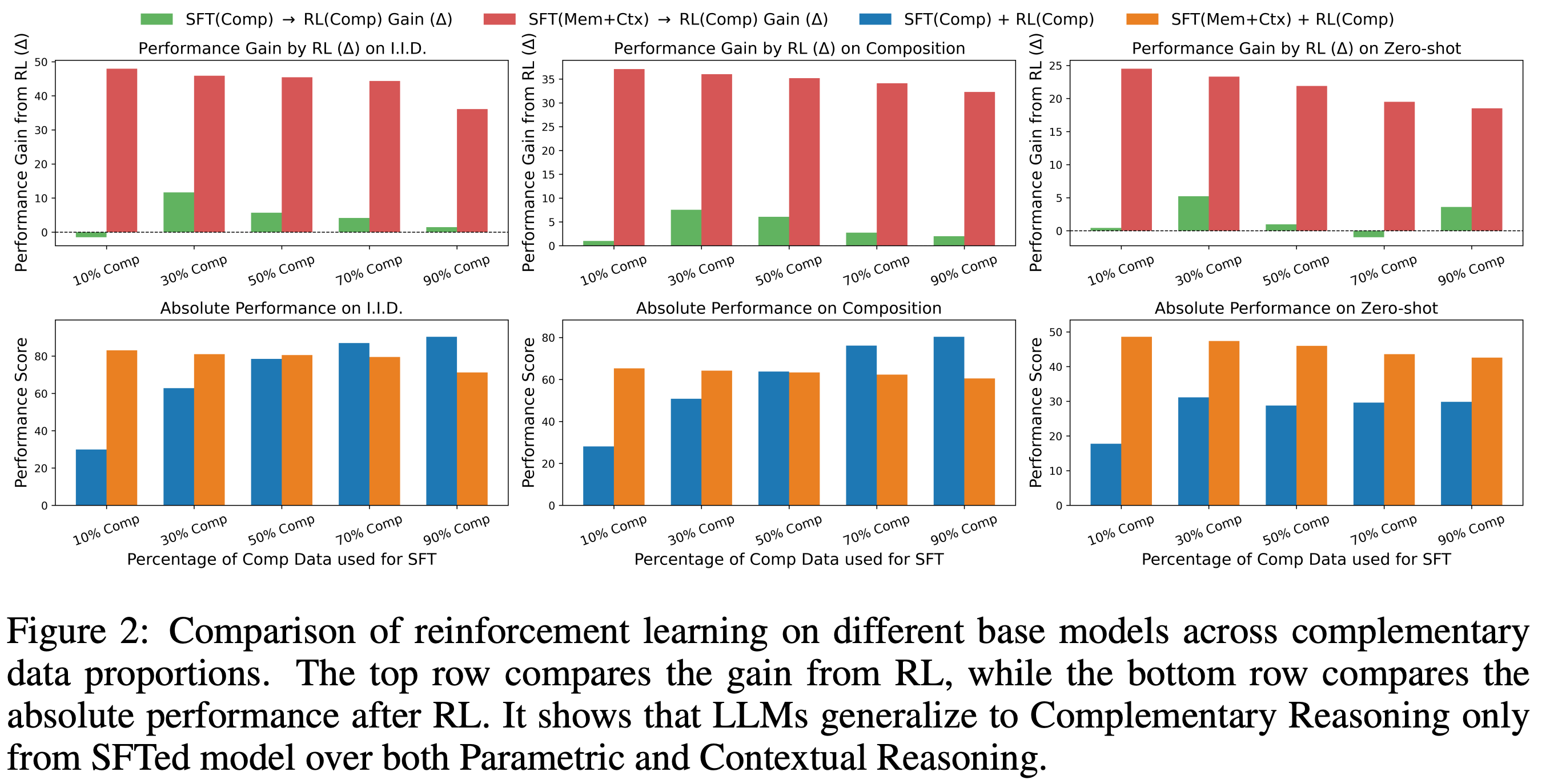
As we can see, this analysis shows us that RL is capable of synthesizing multiple atomic reasoning capabilities into higher-level (composite) reasoning patterns. However, this is only possible when the model is trained with SFT prior to RL. In contrast, pure SFT training yields high in-domain performance and poor out-of-domain generalization, which reflects findings in prior work. In other words, SFT tends to memorize reasoning patterns rather than learn them. When a model is first trained via SFT to acquire primitive reasoning capabilities, then RL serves as a “synthesizer” through which the model learns how to properly combine these capabilities for solving complex, compositional reasoning problems.
“[We demonstrate] that RL synthesizes novel reasoning strategies and enables robust zero-shot generalization when LLMs are first pre-trained on foundational atomic reasoning skills via Supervised Fine-Tuning.” - from [8]
Does math reasoning improve general capabilities? A large-scale empirical analysis is performed in [9] to determine whether math-oriented reasoning training is also helpful in other domains. This analysis includes both a wide audit of existing models across math reasoning, general reasoning, and non-reasoning benchmarks, as well as a comparison of SFT and RL-based finetuning on Math-only data (i.e., ~47K prompts sourced from DeepScaler and SimpleRL).
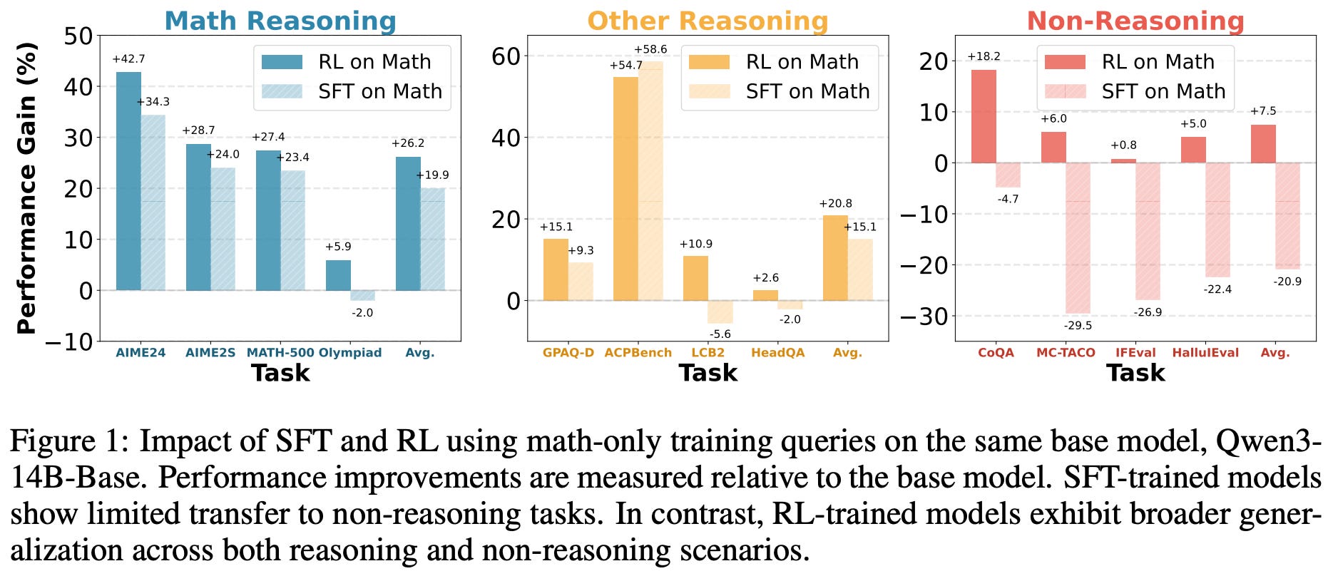
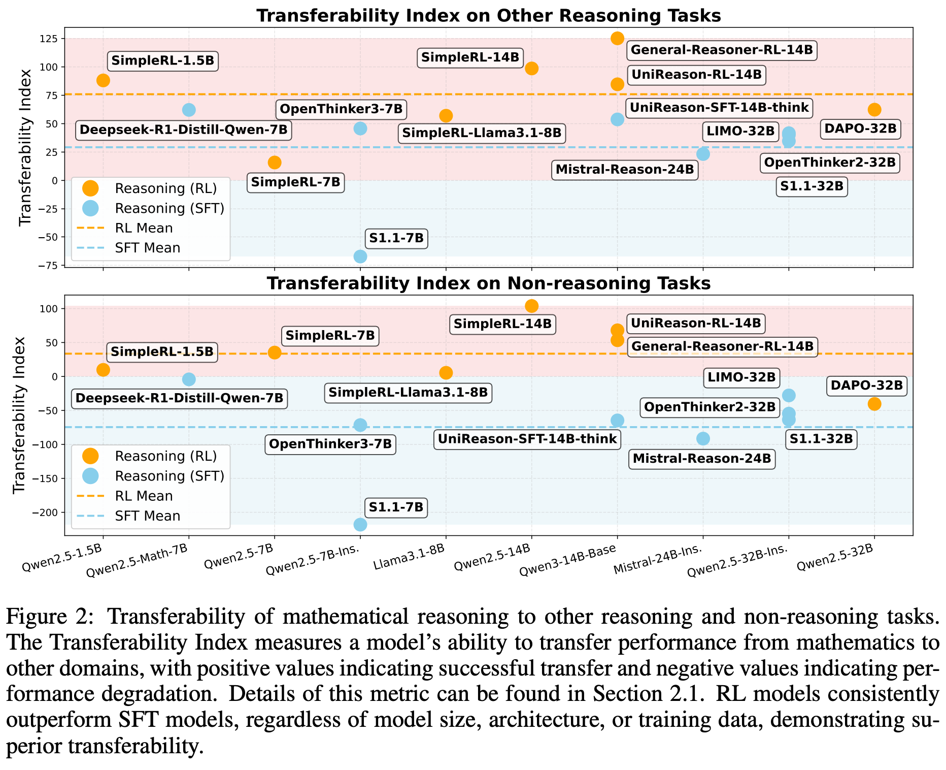
As shown in the above plot, SFT-trained models tend to have poor transferability to non-reasoning tasks, while models trained with RL generalize across both reasoning and non-reasoning tasks—RL models generalize well beyond math and naturally avoid catastrophic forgetting. Similar trends are observed when analyzing the transferability of other open SFT or reasoning models across reasoning and non-reasoning benchmarks; see below. Further analysis in [9] reveals that on-policy data—as we might expect from [2, 3]—and the presence of a negative gradient in the RL objective are key contributors to favorable generalization properties.
Conclusion
In continual learning, we want the model to learn new tasks quickly while preserving old capabilities. When studying recent work on continual learning for LLMs, a consistent pattern emerges: on-policy RL is naturally more robust to catastrophic forgetting relative to SFT, even without explicit mechanisms to aid the continual learning process. This advantage appears to stem from the online nature of RL, which biases learning toward low distribution shift (or low KL) solutions and avoids destructive updates induced by offline data. The natural continual learning abilities of RL have broader implications for the emergence of AGI, as adaptability is a key prerequisite for generally intelligent systems. The studies seen in this overview use only simple, structured proxies for continual learning in the real world, which will be much messier. However, these results show that RL—an already impactful training paradigm—is a promising starting point for building general systems that can adapt to any task. In this way, continuing the existing trajectory of LLM research may yield natural progress for continual learning.
New to the newsletter?
Hi! I’m Cameron R. Wolfe, Deep Learning Ph.D. and Senior Research Scientist at Netflix. This is the Deep (Learning) Focus newsletter, where I help readers better understand important topics in AI research. The newsletter will always be free and open to read. If you like the newsletter, please subscribe, consider a paid subscription, share it, or follow me on X and LinkedIn!
Bibliography
[1] Lai, Song, et al. “Reinforcement fine-tuning naturally mitigates forgetting in continual post-training.” arXiv preprint arXiv:2507.05386 (2025).
[2] Chen, Howard, et al. “Retaining by doing: The role of on-policy data in mitigating forgetting.” arXiv preprint arXiv:2510.18874 (2025).
[3] Shenfeld, Idan, Jyothish Pari, and Pulkit Agrawal. “Rl’s razor: Why online reinforcement learning forgets less.” arXiv preprint arXiv:2509.04259 (2025).
[4] Lu, Kevin et al. “On-Policy Distillation.” https://thinkingmachines.ai/blog/on-policy-distillation/ (2025).
[5] Meng, Yu, Mengzhou Xia, and Danqi Chen. “Simpo: Simple preference optimization with a reference-free reward.” Advances in Neural Information Processing Systems 37 (2024): 124198-124235.
[6] Diao, Muxi, et al. “Entropy-Adaptive Fine-Tuning: Resolving Confident Conflicts to Mitigate Forgetting.” arXiv preprint arXiv:2601.02151 (2026).
[7] Chu, Tianzhe, et al. “Sft memorizes, rl generalizes: A comparative study of foundation model post-training.” arXiv preprint arXiv:2501.17161 (2025).
[8] Cheng, Sitao, et al. “From Atomic to Composite: Reinforcement Learning Enables Generalization in Complementary Reasoning.” arXiv preprint arXiv:2512.01970 (2025).
[9] Huan, Maggie, et al. “Does Math Reasoning Improve General LLM Capabilities? Understanding Transferability of LLM Reasoning.” arXiv preprint arXiv:2507.00432 (2025).
[10] McCloskey, Michael, and Neal J. Cohen. “Catastrophic interference in connectionist networks: The sequential learning problem.” Psychology of learning and motivation. Vol. 24. Academic Press, 1989. 109-165.
[11] Kirkpatrick, James, et al. “Overcoming catastrophic forgetting in neural networks.” Proceedings of the national academy of sciences 114.13 (2017): 3521-3526.
[12] Rebuffi, Sylvestre-Alvise, et al. “icarl: Incremental classifier and representation learning.” Proceedings of the IEEE conference on Computer Vision and Pattern Recognition. 2017.
[13] Castro, Francisco M., et al. “End-to-end incremental learning.” Proceedings of the European conference on computer vision (ECCV). 2018.
[14] Chaudhry, Arslan, et al. “On tiny episodic memories in continual learning.” arXiv preprint arXiv:1902.10486 (2019).
[15] Hayes, Tyler L., et al. “Remind your neural network to prevent catastrophic forgetting.” European conference on computer vision. Cham: Springer International Publishing, 2020.
[16] Rannen, Amal, et al. “Encoder based lifelong learning.” Proceedings of the IEEE international conference on computer vision. 2017.
[17] Shin, Hanul, et al. “Continual learning with deep generative replay.” Advances in neural information processing systems 30 (2017).
[18] Hinton, Geoffrey, Oriol Vinyals, and Jeff Dean. “Distilling the knowledge in a neural network.” arXiv preprint arXiv:1503.02531 (2015).
[19] Li, Zhizhong, and Derek Hoiem. “Learning without forgetting.” IEEE transactions on pattern analysis and machine intelligence 40.12 (2017): 2935-2947.
[20] Wu, Yue, et al. “Large scale incremental learning.” Proceedings of the IEEE/CVF conference on computer vision and pattern recognition. 2019.
[21] Aljundi, Rahaf, et al. “Memory aware synapses: Learning what (not) to forget.” Proceedings of the European conference on computer vision (ECCV). 2018.
[22] Dhar, Prithviraj, et al. “Learning without memorizing.” Proceedings of the IEEE/CVF conference on computer vision and pattern recognition. 2019.
[24] Rusu, Andrei A., et al. “Progressive neural networks.” arXiv preprint arXiv:1606.04671 (2016).
[25] Draelos, Timothy J., et al. “Neurogenesis deep learning: Extending deep networks to accommodate new classes.” 2017 international joint conference on neural networks (IJCNN). IEEE, 2017.
[26] Guo, Haiyang, et al. “Hide-llava: Hierarchical decoupling for continual instruction tuning of multimodal large language model.” arXiv preprint arXiv:2503.12941 (2025).
[27] Zhao, Hongbo, et al. “Mllm-cl: Continual learning for multimodal large language models.” arXiv preprint arXiv:2506.05453 (2025).
[28] Li, Hongbo, et al. “Theory on mixture-of-experts in continual learning.” arXiv preprint arXiv:2406.16437 (2024).
[29] Liu, Wenzhuo, et al. “LLaVA-c: Continual Improved Visual Instruction Tuning.” arXiv preprint arXiv:2506.08666 (2025).
[30] Maharana, Adyasha, et al. “Adapt-$\infty $: Scalable continual multimodal instruction tuning via dynamic data selection.” arXiv preprint arXiv:2410.10636 (2024).
[31] Lee, Minjae, et al. “OASIS: Online Sample Selection for Continual Visual Instruction Tuning.” arXiv preprint arXiv:2506.02011 (2025).
Earlier research papers on this topic also commonly use the term “catastrophic interference” to refer to the same concept as catastrophic forgetting.
The reference model is usually the initial policy prior to RL training, such as the SFT model or a base model.
See Section 2.1 of this paper for an exact explanation of how entropy is computed using token probabilities outputted by an LLM.
More specifically, authors in [1] mention that, without any KL divergence term, the RL training process has to be resumed after a divergence numerous times for the final model to converge properly.
This is a play on words related to the concept of Occam’s Razor, which suggests that the simplest solution (or the solution requiring the fewest assumptions or elements) is usually correct.
For example, if we want to reduce the amount of forgetting when training with SFT, we can simply lower our learning rate [2].
stellar work as always, thank you.
I didn't know about the forward and reverse KL divergences and https://huggingface.co/blog/NormalUhr/kl-divergence-estimator-rl-llm was also very interesting, thank you for the link!
RL also involves fewer bits of information than SFT. So how do you fairly compare them?