GRPO++: Tricks for Making RL Actually Work

How to go from the vanilla GRPO algorithm to functional RL training at scale...

(from [1, 3, 4])

Recent research on large language models (LLMs) has been heavily focused on reasoning and reinforcement learning (RL). At the center of this research lies Group Relative Policy Optimization (GRPO) [13], the RL optimizer used to train most open-source reasoning models. The popularity of GRPO is enhanced by its conceptual simplicity and practical efficiency. However, the simplicity of GRPO can be deceptive—the vanilla GRPO algorithm has subtle issues that can hinder the RL training process, especially at scale. Solving the shortcomings of GRPO has become a popular research topic, leading to the proposal of many tricks, best practices, and techniques for getting the most out of RL training. In this overview, we will outline all of this work, arriving at a deeper practical understanding of how to modify and use GRPO for training high-quality reasoning models.

Background on Reasoning and RL

Prior to covering recent work on improving GRPO, we will spend this section building a basic understanding of the GRPO algorithm in its original form. We will also learn about Proximal Policy Optimization (PPO) [11], the predecessor to GRPO, and discuss how RL is used in the context of LLMs and reasoning models more generally. Notably, this discussion will assume basic knowledge of the problem setup and terminology used for RL training with LLMs. Those who are less familiar with RL basics can learn more at the following links:

• RL Problem Setup & Terminology [link]

• Different RL Formulations for LLMs [link]

• Policy Gradient Basics [link]

RL for Reasoning

“Inference scaling empowers LLMs with unprecedented reasoning ability, with RL as the core technique to elicit complex reasoning.” - from [1]

GRPO is the most common RL optimizer to use for training reasoning models. Before diving deeper into the details of GRPO, we need to build an understanding of how RL is actually used to train LLMs. In particular, there are two key types of RL training that are commonly used:

• Reinforcement Learning from Human Feedback (RLHF) trains the LLM using RL with rewards derived from a reward model trained on human preferences.

• Reinforcement Learning with Verifiable Rewards (RLVR) trains the LLM using RL with rewards derived from rule-based or deterministic verifiers.

The main difference between RLHF and RLVR is how we assign rewards—RLHF uses a reward model, while RLVR uses verifiable rewards. Aside from this difference, both are online RL algorithms with a similar structure; see below. GRPO is one possible RL optimizer that can be used to derive the policy update in this pipeline, though any RL optimizer (e.g., PPO or REINFORCE) can be used.

General framework for online RL

Given that RLHF focuses on aligning an LLM to human preferences, it is used more heavily for chat models and is less applicable to reasoning¹. Most reasoning models are trained using RL in verifiable domains (e.g., math and coding), so we will primarily focus on the RLVR setup for the remainder of this post.

More on RLVR. To train an LLM with RLVR, we must select a domain that is verifiable in nature; e.g., math or coding. In other words, we need to create a dataset that has either i) a known ground truth answer or ii) some rule-based technique that can be used to verify the correctness of responses to the prompts in our dataset. For coding, we can create a sandbox for running LLM-generated code and use test cases to assess correctness. Similarly, we can evaluate math problems by performing basic string matching between the answer predicted by the LLM and a ground-truth answer for a problem; see below.

Verifying a problem with exact string matching

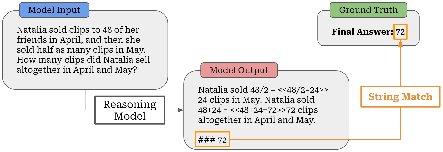
Usually, we must instruct the LLM to format its output so the final answer can be easily parsed. As an example, Math Verify is a popular package that was built for performing robust verification in the math domain. Even then, however, string matching is not always sufficient for evaluating correctness. In many cases, we can benefit from crafting validation logic that is more robust (e.g., asking an LLM to identify equivalent answers) and that captures variations in output.

“Math verification is determined by an LLM judge given the ground truth solution and DeepSeek-R1 solution attempt. We found that using an LLM judge instead of a stricter parsing engine (Math-Verify) for verification during data generation results in a higher yield and leads to higher performing downstream models.” - source

Reasoning models are structurally identical to a standard LLM. The key distinction between reasoning models and LLMs is the ability to “think” about a prompt prior to providing a final output. By increasing the length of this thinking process, reasoning models can use inference-time scaling—or simply spend more compute on generating a particular completion—to improve their performance.

Concrete example of a reasoning model’s full output

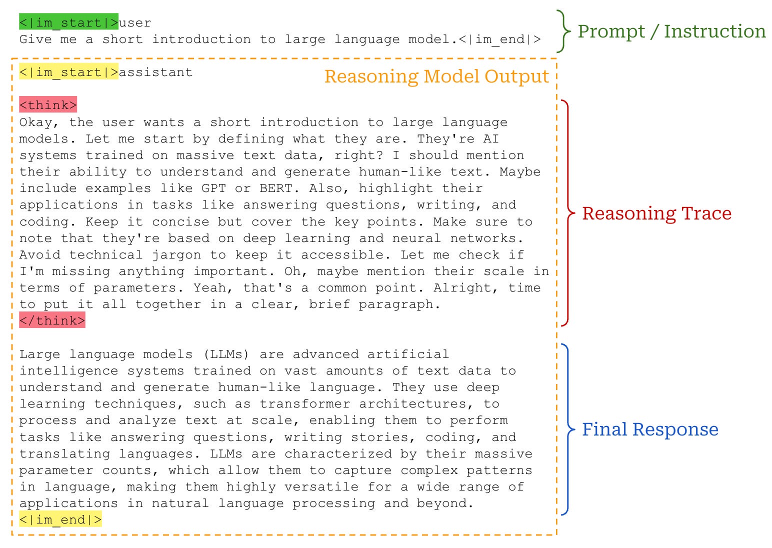
As shown above, this thinking process occurs in the form of a free-text, long chain-of-thought (CoT)—also called a rationale or reasoning trajectory—generated by the LLM. Many closed reasoning models (though not all of them!) hide the raw reasoning trace from the user, providing instead only a truncated version or summary of the reasoning process along with the model’s final answer.

Learning to reason via RL. If we look at some examples of reasoning trajectories from open or closed reasoning models, we will notice that these models exhibit some sophisticated reasoning behaviors in their long CoT:

• Thinking through each part of a complex problem.

• Decomposing complex problems into smaller, solvable parts.

• Critiquing solutions and finding errors.

• Exploring many alternative solutions.

Such behavior goes beyond any previously-observed behavior with standard LLMs and chain of thought prompting. However, this behavior is not explicitly injected into the model—it is naturally developed via large-scale RL training!

“One of the most remarkable aspects of this self-evolution is the emergence of sophisticated behaviors as the test-time computation increases. Behaviors such as reflection—where the model revisits and reevaluates its previous steps—and the exploration of alternative approaches to problem-solving arise spontaneously. These behaviors are not explicitly programmed but instead emerge as a result of the model’s interaction with the reinforcement learning environment.” - from [2]

During RLVR, the model undergoes a self-exploration process in which it learns how to properly use its long CoT to solve reasoning problems. As evidence of this self-evolution process, we commonly observe during RL training that the average length of the model’s completions increases over time; see below. The model naturally learns how to use more inference-time compute (by generating a longer reasoning trace) in order to solve difficult reasoning problems.

(from [2])

Training stages and Aha moments. As shown below, LLMs undergo training in several stages. However, reasoning models depart from the standard alignment procedure—including supervised finetuning (SFT) and RLHF—by adding an extra RLVR training stage. Additionally, it is even common in RL research to use an RL-Zero setup in which we directly train the pretrained base model with RLVR.

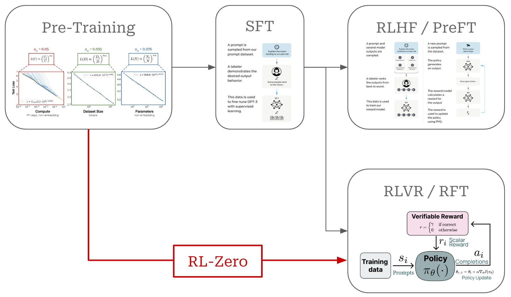
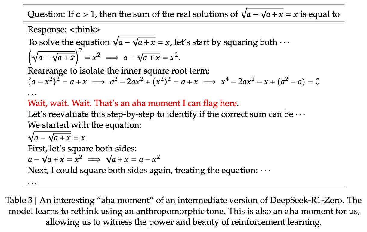
The RL-Zero setup was popularized by DeepSeek-R1 [2], which showed that reasoning capabilities can be instilled in an LLM via pure RL (using GRPO) even with no SFT. Most notably, DeepSeek-R1-Zero—the version of DeepSeek-R1 that is trained with an RL-Zero setup—is found in [2] to have an “Aha moment” in which it learns to invest additional reasoning effort into re-thinking or evaluating its own responses inside of the reasoning trace; see below. This behavior emerges at an intermediate point in RL training and is a classic example of how self-exploration via RL can naturally lead an LLM to develop sophisticated reasoning behavior.

(from [2])

Proximal Policy Optimization (PPO)

GRPO is based on the Proximal Policy Optimization (PPO) algorithm [11]. PPO was used in seminal work on RLHF and, as a result, was the default RL optimizer in the LLM domain for some time. Only after the advent of reasoning models did alternative algorithms like GRPO begin to gain traction for training LLMs. A full overview of PPO is linked below, but we will cover the key details in this section.

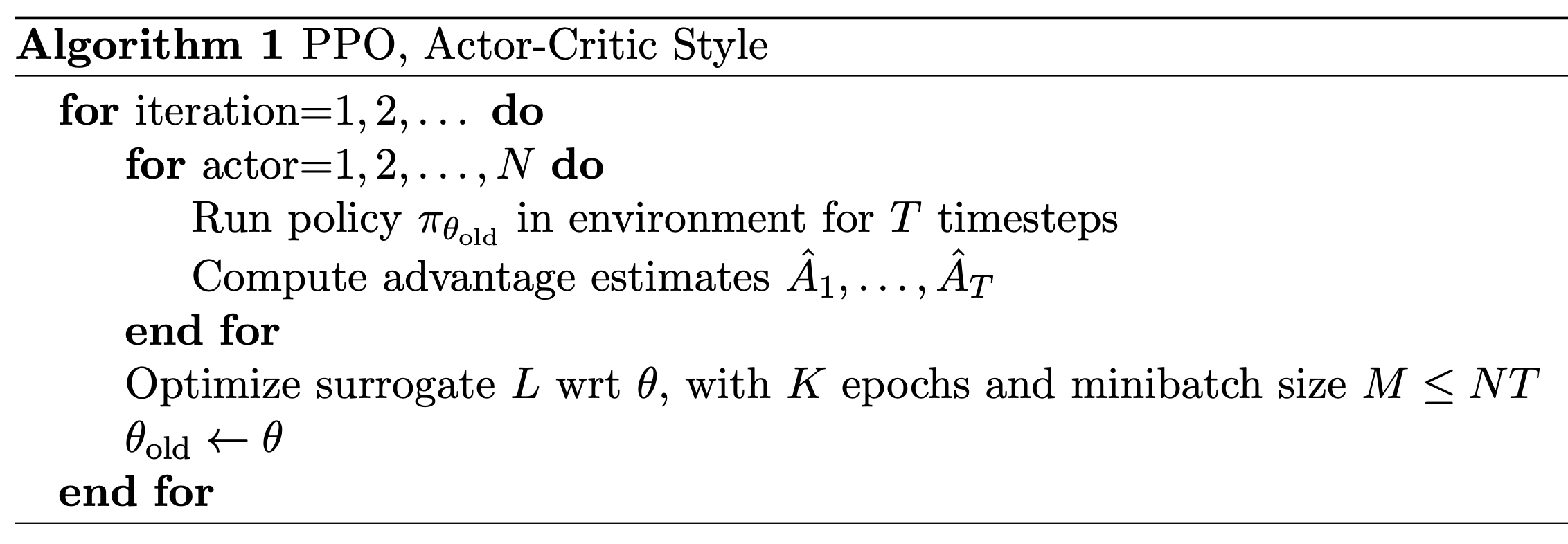
The structure of training with PPO is outlined below. As we can see, each training iteration of PPO goes through the following sequence of steps:

1. Sample a diverse batch of prompts.

2. Generate a completion from the policy for each prompt.

3. Compute advantage estimates for each completion.

4. Perform several policy updates over this sampled data.

(from [11])

Surrogate objective. In PPO, we formulate a loss function (also called the surrogate objective) that is optimized with respect to the parameters of our policy. The PPO loss function is based on the policy ratio (also called the importance ratio) between the current and “old” (i.e., before the first update in a training step) policies. The importance ratio stabilizes the training process by comparing the new policy’s token probabilities to the old policy and applying a weight (or importance) to training that helps to avoid drastic changes; see below.

Policy or importance ratio

To derive the surrogate objective for PPO, we begin with an unclipped objective that resembles the surrogate objective used in Trust Region Policy Optimization (TRPO); see below. Additionally, we introduce a clipped version of this objective by applying a clipping mechanism to the policy ratio r_t(θ). Clipping forces the policy ratio to fall in the range [1 - ε, 1 + ε]. In other words, we avoid the policy ratio becoming too large or too small, ensuring that the token probabilities produced by the current and old policies remain relatively similar.

The PPO surrogate objective

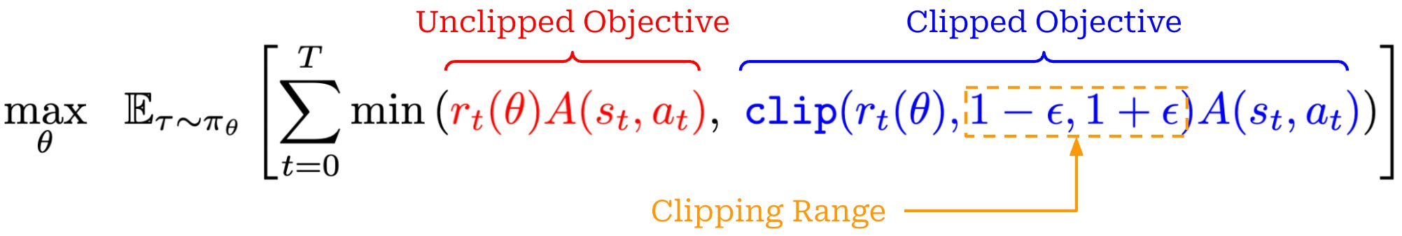
The PPO surrogate objective is simply the minimum of clipped and unclipped objectives, which makes it a pessimistic (lower bound) estimate for the unclipped objective. The behavior of the clipping mechanism in the surrogate loss changes depending on the sign of the advantage. The possible cases are shown below.

(from [11])

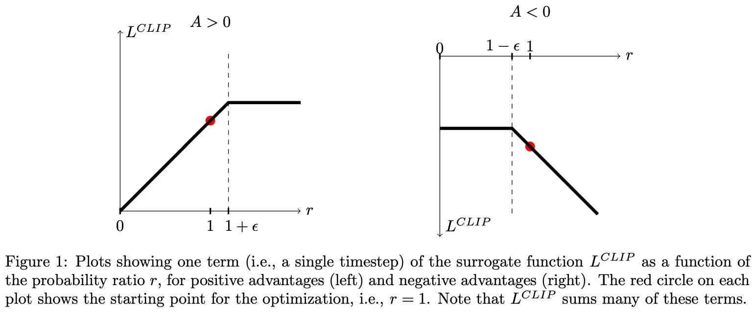
As we can see, taking the minimum of clipped and unclipped terms in the surrogate objective causes clipping to be applied in only one direction. The surrogate objective can be arbitrarily decreased by moving the importance ratio away from one, but clipping prevents the objective from being increased beyond a certain point by limiting the importance ratio. In this way, the clipping in PPO disincentivizes large policy ratios and, in turn, maintains a trust region by preventing large policy updates that could potentially damage our policy.

“We only ignore the change in probability ratio when it would make the objective improve, and we include it when it makes the objective worse.” - from [11]

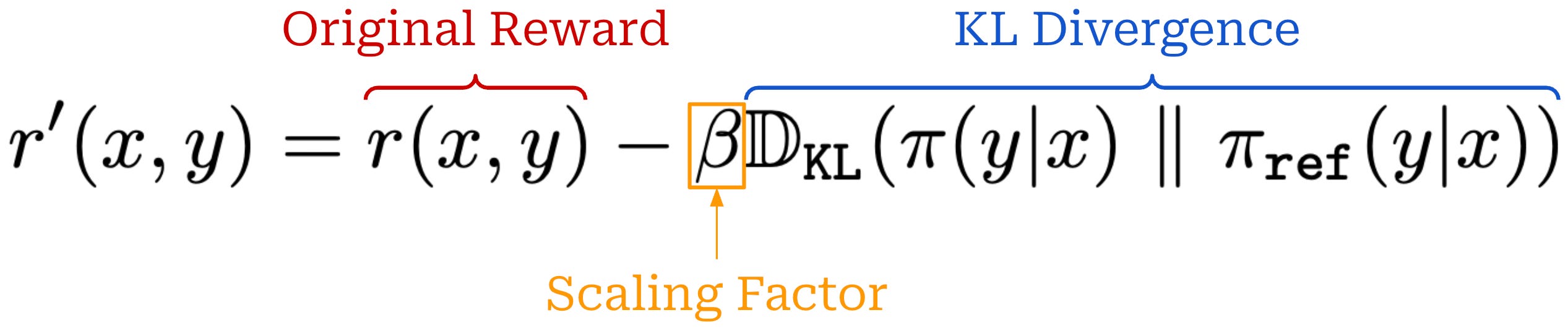
KL divergence. We often incorporate a KL divergence between the current policy and a reference policy—usually the model from the beginning of training—into RL. The KL divergence serves as a penalty that encourages similarity between the current and reference policies. We compute the KL divergence by comparing token distributions from the two LLMs for each token in a sequence. The easiest—and most common—way to approximate KL divergence [12] is via the difference in log probabilities between the policy and reference; see here.

After the KL divergence has been computed, there are two primary ways that it can be incorporated into the RL training process:

1. By directly subtracting the KL divergence from the reward.

2. By adding the KL divergence to the loss function as a penalty term.

PPO adopts the former option by subtracting the KL divergence directly from the reward signal used in RL training, as shown in the equation below.

Adding KL divergence to the reward in PPO

Advantage estimation. The advantage function, a key part of PPO’s surrogate objective, is the difference between the action-value and value function: A(s, a) = Q(s, a) - V(s). The value function in PPO is estimated with a learned model called the value model (or critic). This critic is a separate copy of our policy, or—for better parameter efficiency—an added value head that shares weights with the policy. The critic takes a completion as input and predicts expected cumulative reward on a per-token basis using an architecture that is similar to that of a reward model (i.e., transformer with a regression head); see below.

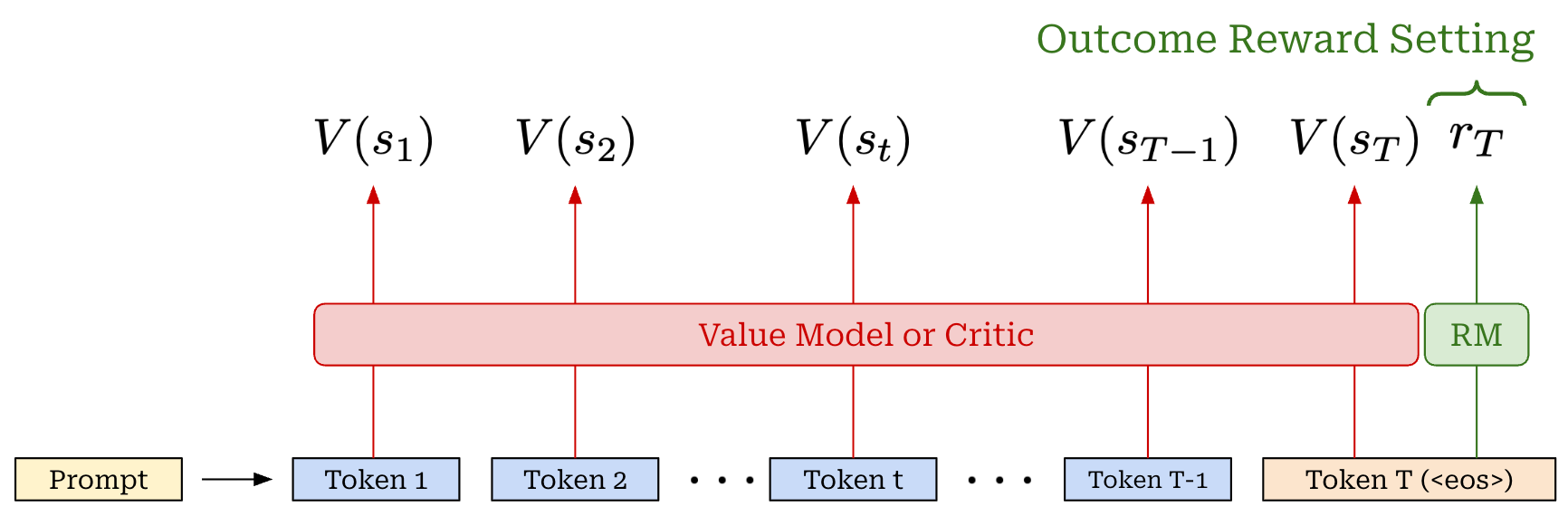
The value function is on-policy—it depends on the current parameters of our policy. Unlike reward models, which are fixed at the beginning of RL training, the critic is trained alongside the LLM to keep its predictions on-policy—this is known as an actor-critic setup. To train the critic, we add an extra mean-squared error (MSE) loss term—between the rewards predicted by the critic and the actual rewards—to the PPO loss. Using the critic, we can estimate advantage using Generalized Advantage Estimation (GAE). The details of GAE are beyond the scope of this post, but a full explanation and implementation can be found here.

Group Relative Policy Optimization (GRPO)

(from [13])

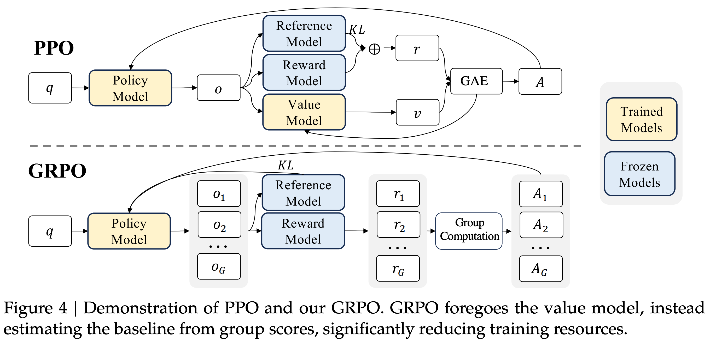
Group Relative Policy Optimization (GRPO) [13] builds upon PPO by proposing a simpler technique for estimating the advantage. In particular, GRPO estimates the advantage by sampling multiple completions—or a “group” of completions—for each prompt and using the rewards of these completions to form a baseline. This group-derived baseline replaces the value function, which allows GRPO to forgo training a critic. Avoiding the critic drastically reduces GRPO’s memory and compute overhead compared to PPO. Additionally, since GRPO is commonly used for reasoning-oriented training, we typically pair it with verifiable rewards, which eliminates the need for a separate reward model.

“We introduce the Group Relative Policy Optimization (GRPO), a variant of Proximal Policy Optimization (PPO). GRPO foregoes the critic model, instead estimating the baseline from group scores, significantly reducing training resources.” - from [13]

Advantage estimation in GRPO is performed by sampling multiple completions for each prompt and using the formulation shown below. This approach is very simple compared to PPO, which uses a learned value model and GAE.

Advantage computation in GRPO

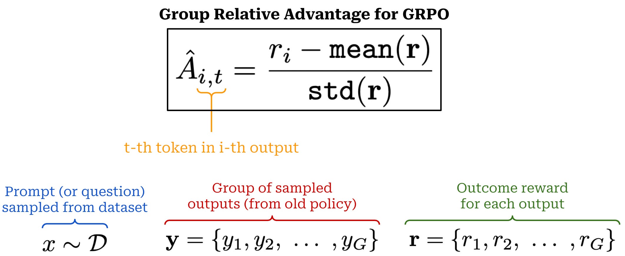
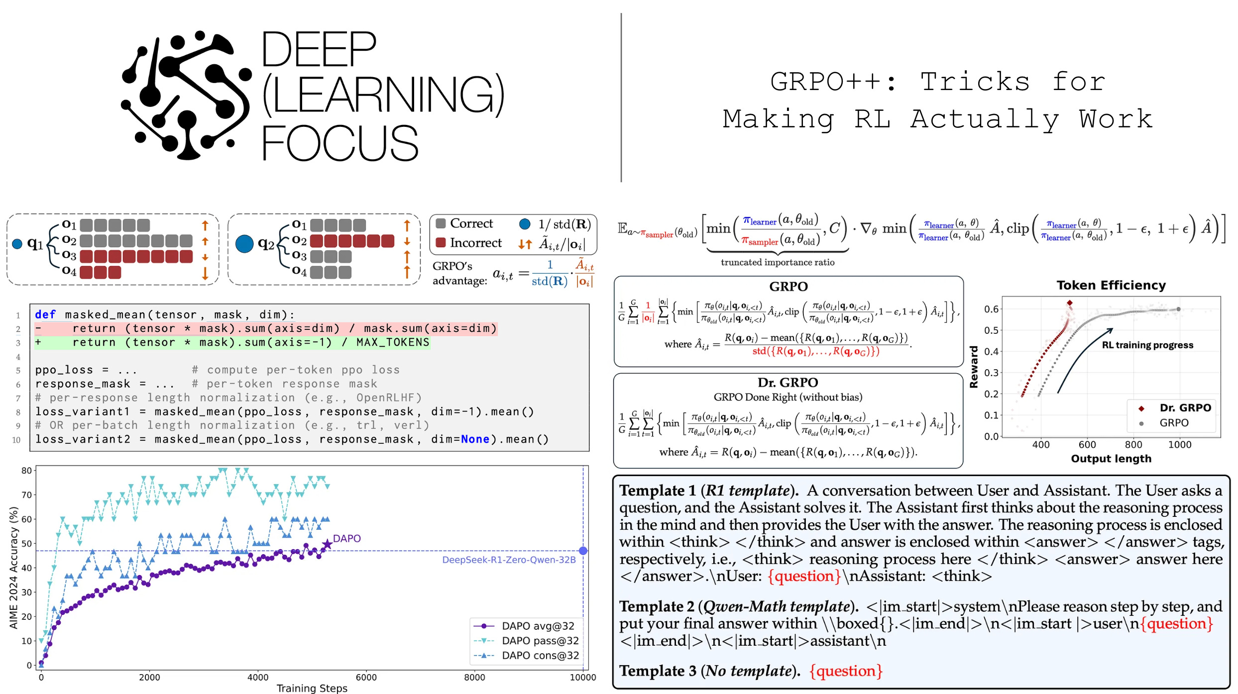
In GRPO, completions to the same prompt form a group, and we calculate the advantage relative to other rewards in the group—hence, the name “group relative” policy optimization! More specifically, the advantage for completion i is calculated by first subtracting the mean reward over the group from r_i, then dividing this difference by the standard deviation of rewards over the group. The GRPO loss is assigned on a per-token basis, but we should note that the above formulation assigns the same advantage to every token t in completion i. The per-token loss is therefore dictated by the policy ratio, which varies for each token.

“GRPO is often run with a far higher number of samples per prompt because the advantage is entirely about the relative value of a completion to its peers from that prompt.” - RLHF book

Because we compute the advantage in a relative manner (i.e., based on rewards in the group), the number of completions we sample per prompt must be high to obtain a stable policy gradient estimate. Unlike GRPO, PPO and REINFORCE typically sample a single completion per prompt. However, sampling multiple completions per prompt has been explored by prior RL optimizers like RLOO.

Surrogate loss. Despite estimating the advantage differently, GRPO uses a loss function that is nearly identical to that of PPO. As shown below, GRPO uses the same clipping mechanism that is used by PPO for the importance ratio. This expression assumes an MDP formulation and has been modified to explicitly aggregate the loss over multiple completions within a group.

GRPO surrogate loss

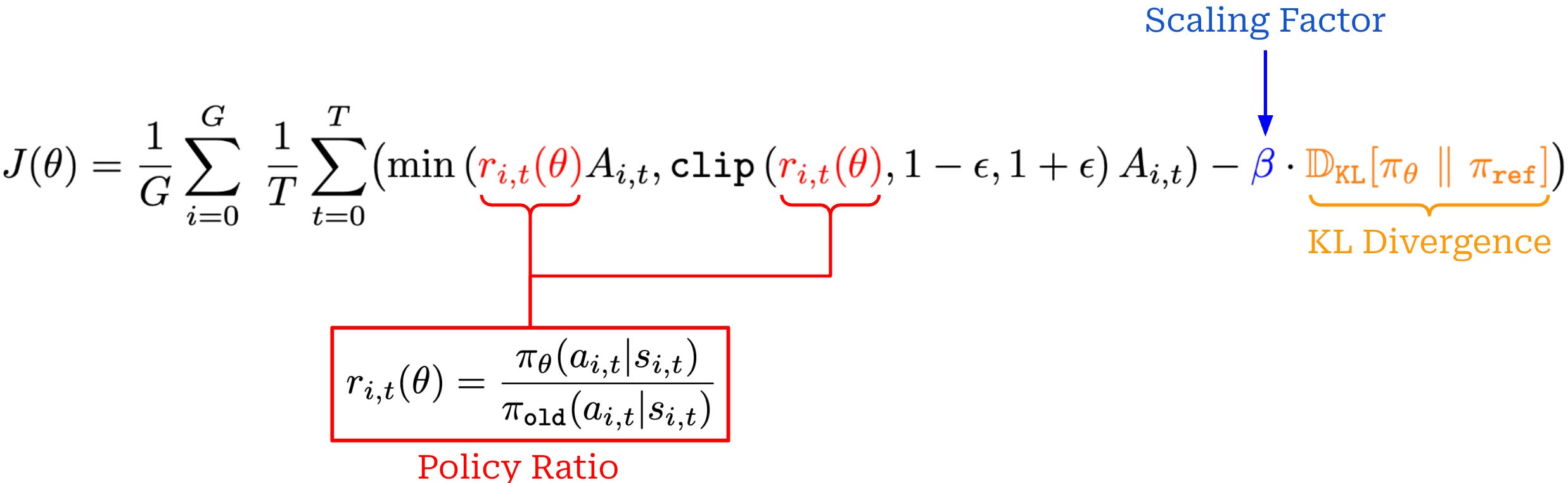
KL divergence. One key difference between PPO and GRPO is the KL divergence term being added as a penalty term to the surrogate loss, rather than subtracted from the reward. However, we should note that the KL divergence is frequently omitted when training reasoning models. In the context of RLHF, KL divergence enables model alignment without diverging significantly from the initial model, but this approach makes less sense when training long CoT reasoning models. The model’s behavior may diverge significantly from the initial model as it develops the ability to perform long CoT reasoning. All of the work that we will study in this overview omits the KL divergence term during RL training.

Limitations of vanilla GRPO. For a full overview of GRPO, please see the above link. As we have seen, GRPO is a relatively simple algorithm. The popularity of GRPO was catalyzed by its use for training DeepSeek-R1 [2]. The openness of this work led GRPO to be adopted in open replications of reasoning models, as well as countless other research efforts. Despite its popularity, vanilla GRPO has several issues that become especially pronounced in large-scale RL training runs:

• Noise and instability during the training process.

• Excessive response lengths, especially in incorrect answers.

• Collapse of the LLM’s entropy (i.e., reduced exploration).

• Poor sample efficiency and slow learning.

Due to these issues, many open research efforts initially struggled to replicate the results reported by DeepSeek-R1 [1, 3], indicating that some details necessary to achieve peak performance with GRPO may have been omitted from [2]. This overview will study various works that have diagnosed such issues with GRPO, uncovering a set of practical tricks that can be used to train better reasoning models at scale.

Assessing the Health of RL Training

Despite the recent success of reasoning models, we must remember that training LLMs via RL is a complex process with many moving parts. We are working with multiple disjoint systems to train the model, each of which has unique settings that must be tuned. As described below, even simple changes to the RL training process can yield unexpected results or completely derail the model. When issues occur, it can be hard to know exactly what went wrong, and the high cost of RL training can make debugging these issues slower and more difficult. To quickly identify issues and iterate on our RL training setup, we need intermediate metrics that allow us to efficiently monitor the health of the training process.

“Reinforcement learning on large language models is… an intrinsically complex systems engineering challenge, characterized by the interdependence of its various subsystems. Modifications to any single subsystem can propagate through the system, leading to unforeseen consequences due to the intricate interplay among these components. Even seemingly minor changes… can amplify through iterative reinforcement learning processes, yielding substantial deviations in outcomes.” - from [1]

Health checks. The key training and policy metrics that can be monitored to catch issues with our RL setup are as follows:

1. Response length should increase during reasoning RL as the policy learns how to effectively leverage its long CoT. Average response length is closely related to training stability, but response length does not always monotonically increase—it may stagnate or even decrease. Excessively long response lengths are also a symptom of a faulty RL setup.

2. Training reward should increase in a stable manner throughout training. A noisy or chaotic reward curve is a clear sign of an issue in our RL setup. However, training rewards do not always accurately reflect the model’s performance on held-out data—RL tends to overfit to the training set.

3. Entropy² of the policy’s next token prediction distribution serves as a proxy for exploration during RL training. We want entropy to lie in a reasonable range—not too low and not too high. Low entropy means that the next token distribution is too sharp (i.e., all probability is assigned to a single token), which limits exploration. On the other hand, entropy that is too high may indicate the policy is just outputting gibberish. Similarly to entropy, we can also monitor the model’s generation probabilities during RL training.

4. Held-out evaluation should be performed to track our policy’s performance (e.g., average reward or accuracy) as training progresses. Performance should be monitored specifically on held-out validation data to ensure that no reward hacking is taking place. This validation set can be kept (relatively) small to avoid reducing the efficiency of the training process.

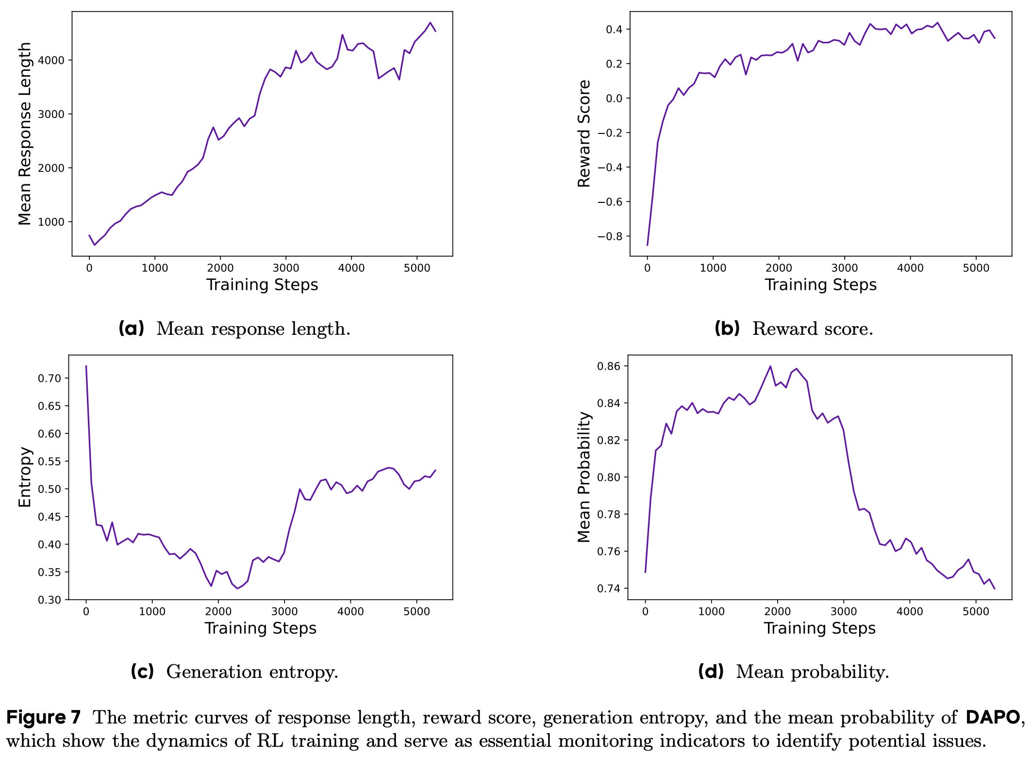
An example plot of these key intermediate metrics throughout the RL training process from DAPO [1] is shown below. To iterate upon our RL training setup, we should i) begin with a reasonable setup known to work well, ii) apply interventions to this setup, and iii) monitor these metrics for positive or negative impact. We will see many examples of such a workflow throughout this overview as we study various tweaks and improvements to the vanilla GRPO algorithm.

“We typically use length in conjunction with validation accuracy as indicators to assess whether an experiment is deteriorating… the trend of reward increase [should be] relatively stable and does not fluctuate or decline significantly due to adjustments in experimental settings… we find that maintaining a slow upward trend in entropy is conducive to the improvement of model performance.” - from [1]

(from [1])

A note on batching and data. Prior to making algorithmic changes to GRPO, we should focus on the correctness of our data. GRPO needs (relatively) large batch sizes to work well. Using a small batch size in GRPO is one of the most common mistakes in RL training. To avoid this mistake, we should begin with a reasonable batch and group size (e.g., Olmo 3 [5] uses a batch size of 512 with 64 prompts and 8 rollouts per prompt) and test how varying the batch and group sizes impacts the metrics discussed above. For example, if a larger batch size makes our reward curve much more stable, then our initial batch size was probably too small.

As shown in recent RL research [9, 10], curating the correct set of prompts is also essential. More specifically, we want our data to be diverse in terms of topic and difficulty. For example, Olmo 3 [5] incorporates several domains—math, coding, instruction following, and general chat—into RL training and uses offline difficulty filtering to filter out prompts that are too easy or too difficult. Using another LLM to gauge prompt difficulty by measuring Pass@K performance is also a common filtering approach [9]. We see each data point multiple times during RL training, so data curricula³ are less relevant. To make the most of our data, we simply want to ensure sufficient quality and diversity!

“Where algorithmic changes can make models more robust to less balanced data, a crucial part of the current RL training is to have a diversity of difficulties in your data. With large batch sizes, the model should have questions that are trivial, somewhat challenging, and nearly impossible in each batch.” - Nathan Lambert

As a final note, certain categories of questions—specifically those that are easily guessable without any true reasoning—can damage the fidelity of RL training. For example, multiple choice questions can easily be reward hacked if the policy randomly guesses an answer to each question. Therefore, removing this style of easily-guessable questions from RL training is a common practice.

Improving upon Vanilla GRPO

Now that we understand GRPO, we will learn about recent research that has identified (and solved) problems with the vanilla GRPO algorithm. Given the popularity of GRPO, many papers have been published on this topic. We will aim to review this work in a way that is both comprehensive and of sufficient depth. The section will begin with longer overviews of a few popular papers. After the longer overviews, we will provide a wider outline of the topic via shorter paper summaries and an exhaustive list of recent and notable publications.

DAPO: An Open-Source LLM Reinforcement Learning System at Scale [1]

Despite the impressive recent results achieved with reasoning models, many details needed to reproduce these results are concealed. In fact, even open models like DeepSeek-R1 [2] do not provide sufficient technical details to fully reproduce their results. A naive application of GRPO with Qwen-2.5-32B achieves a score of 30% on AIME 2024, underperforming the score of 47% achieved in the DeepSeek-R1 technical report. This difficulty in reproducing the results of DeepSeek-R1 hints at missing details that are necessary for stable, performant, and scalable RL.

“The broader community has encountered similar challenges in reproducing DeepSeek’s results suggesting that critical training details may have been omitted in the R1 paper that are required to develop an industry-level, large-scale, and reproducible RL system.” - from [1]

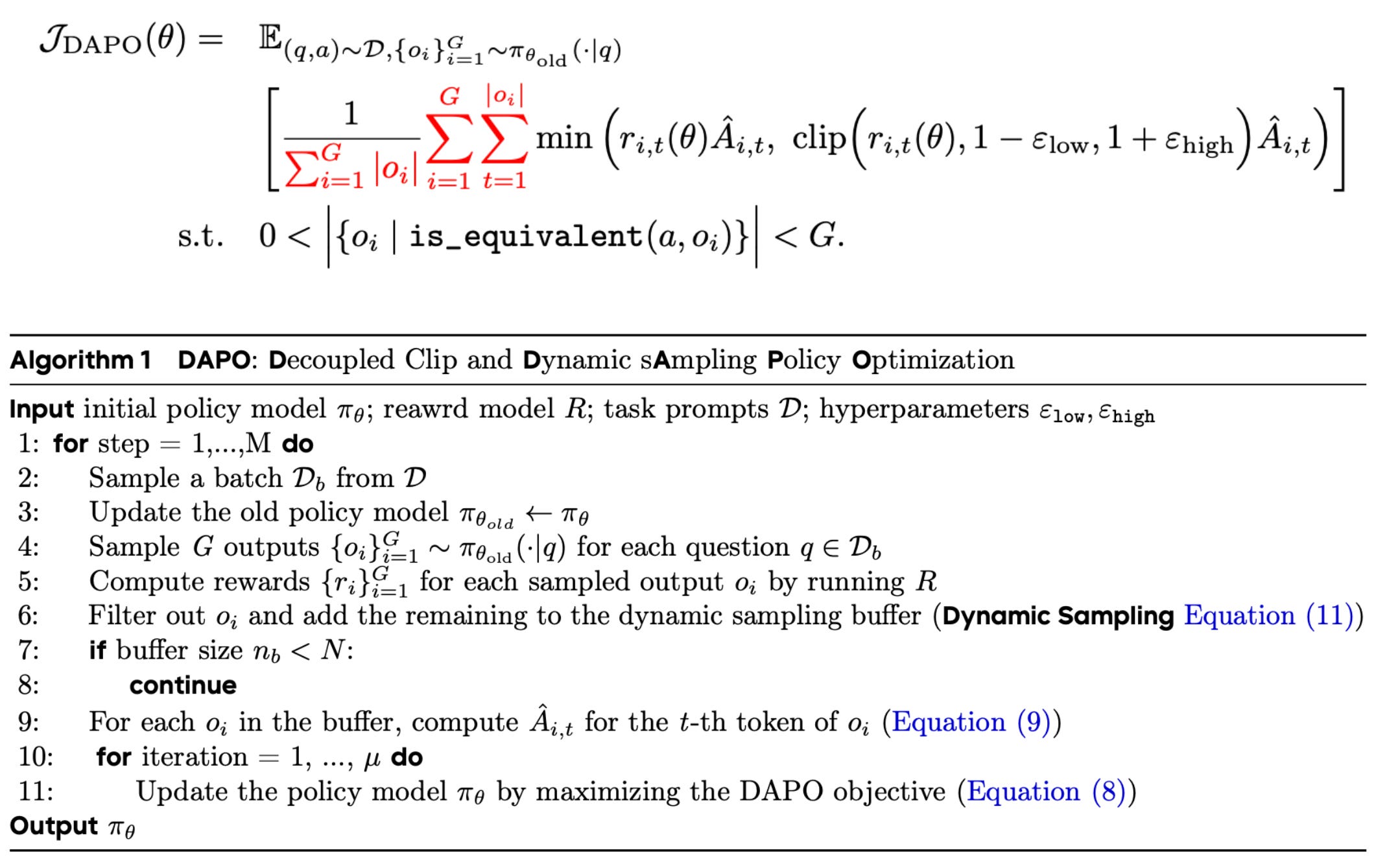
In [1], authors aim to discover these missing details, arriving at four key changes to the vanilla GRPO algorithm that—when applied in tandem—match and surpass results observed in [2]. The modified GRPO algorithm derived in [1] is called the Decoupled Clip and Dynamic Sampling Policy Optimization (DAPO) algorithm. All code (based on verl) and data are openly released to support future research.

Vanilla GRPO. When running the vanilla GRPO algorithm, authors notice several issues in the training process, including:

• Entropy collapse: the entropy of the model’s next token distribution collapses during the training process. Probability mass is primarily assigned to a single token and outputs are more deterministic.

• Reward noise: the training reward is very noisy and does not steadily increase during the RL training process.

• Training instability: the training process is unstable and may diverge. We do not observe a steady increase in response length during training.

To mitigate these issues, authors propose the following four solutions in [1].

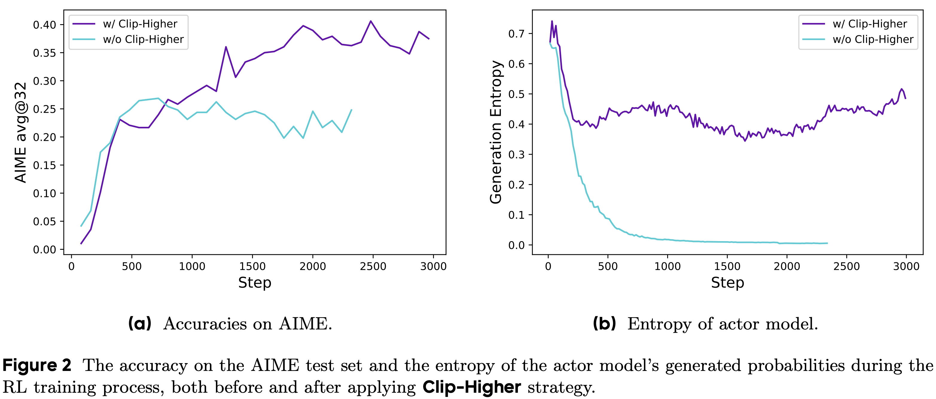
(1) Clip higher. As mentioned previously, authors in [1] observe entropy collapse when training models with vanilla GRPO; see below. When entropy declines, the next token distribution becomes concentrated on a single token, leading sampled responses in a group to be very similar. As a result, exploration becomes limited and the advantage computation in GRPO becomes less reliable—each sample in the group will tend to receive the same reward, making group normalization difficult.

(from [1])

Interestingly, we see in [1] that this entropy collapse is caused by the clipping operation in PPO and GRPO. To see why this occurs, let us consider two kinds of tokens to which clipping could be applied:

1. Exploitation token: a token that is already highly likely in the current policy.

2. Exploration token: a low probability token in the current policy.

Sampling lower probability tokens gives the model a chance to explore alternative tokens when searching for better completions. Clipping is applied to the policy ratio, or the ratio of a token’s probability after and before the policy update:

\(r_t(\theta) = \frac{\pi_\theta(a_t | s_t)}{\pi_{old}(a_t | s_t)}\)

The policy ratio is constrained to a range of [1 - ε, 1 + ε]. This upper bound allows high probability (exploitation) tokens to become more probable, but it restricts increases in low probability (exploration) tokens. A concrete example of how the upper clipping bound can discourage exploration is explained below.

“When ε = 0.2 and [advantage is positive], consider two actions with probabilities π_old(a_t|s_t) = 0.01 and 0.9. The upper bounds of the increased probabilities π_θ(a_t|s_t) are 0.012 and 1.08, respectively (i.e., π_old·(1 + ε)). This implies that exploitation tokens with a higher probability (e.g., 0.9) are not constrained to get even extremely larger probabilities like 0.999. Conversely, for low-probability exploration tokens, achieving a non-trivial increase in probability is considerably more challenging.” - from [1]

The “clip higher” approach, which decouples the lower and upper bound for clipping, is proposed as a solution to this problem. Specifically, we clip in the range [1 - ε_low, 1 + ε_high], where ε_low = 0.2 (default setting) and ε_high = 0.28 in [1]. As shown in the figure above, increasing ε_high prevents entropy collapse and improves GRPO performance. On the other hand, authors note that ε_low should not be increased, as this would suppress some tokens to a probability of zero and collapse the token sampling space.

Ratio of samples with perfect accuracy throughout RL training (from [1])

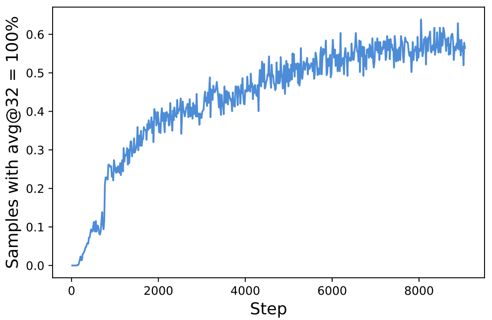
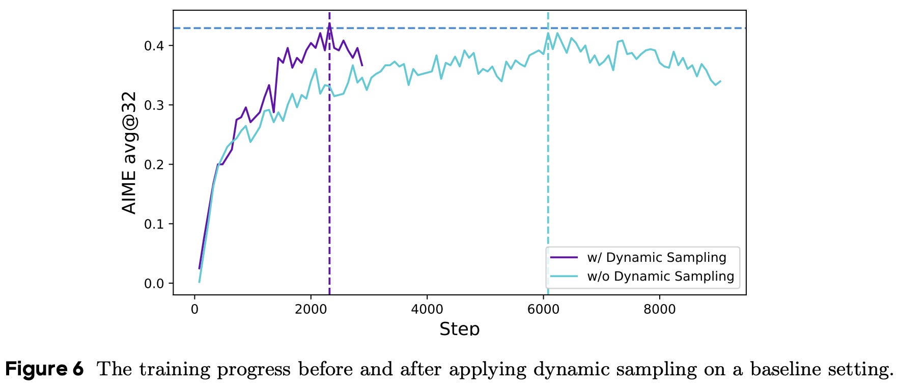
(2) Dynamic Sampling. Throughout the course of RL training, the number of samples for which all completions in a group are correct naturally increases; see above. Although this trend indicates that the model is improving, prompts with perfect accuracy are problematic for GRPO. If all completions in a group are correct (i.e., reward of one), then the advantage for each completion in the group and the corresponding policy gradient are zero. As a result, our batch size effectively becomes smaller because there are many elements in the batch with zero gradient—leading to a noisier batch gradient and, in turn, degraded sample efficiency. To solve this issue, we can perform dynamic sampling, which simply:

1. Over-samples prompts for each batch.

2. Filters or removes all prompts with perfect accuracy.

The sampling cost per batch is dynamic—hence the name “dynamic sampling”—and we simply continue sampling and filtering until we have a full batch. However, this additional sampling cost is typically offset by the improved sample efficiency of the algorithm. Put differently, the model tends to converge much faster when we filter out prompts with perfect accuracy (i.e., dynamic sampling); see below.

(from [1])

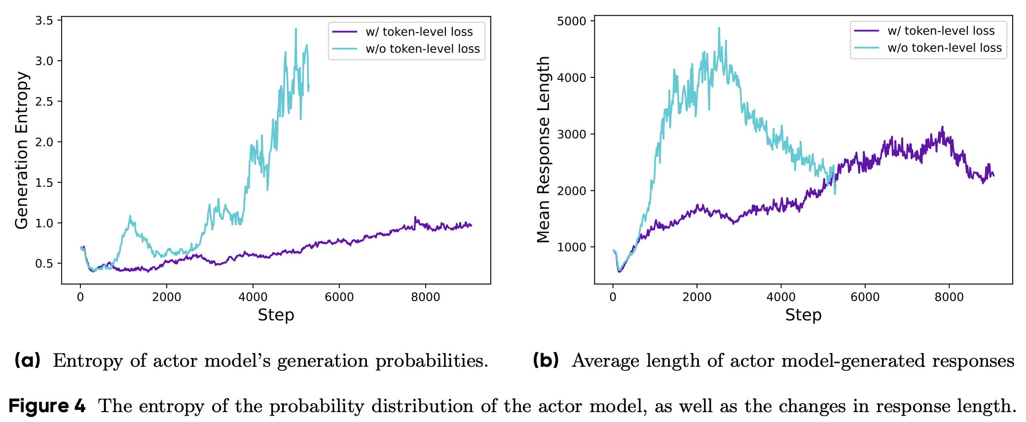
(3) Token-level loss. The GRPO surrogate objective is computed at a token level, but we must aggregate this objective over the batch before computing the policy update. This aggregation is performed at the sample level, as described below.

“The original GRPO algorithm employs a sample-level loss calculation, which involves first averaging the losses by token within each sample and then aggregating the losses across samples. In this approach, each sample is assigned an equal weight in the final loss computation.” - from [1]

When aggregating at the sample level, each sample in the batch is assigned an equal weight in the GRPO loss. Although this approach may seem reasonable, it creates a subtle bias in our GRPO implementation—tokens within long responses have a disproportionately lower contribution to the loss. More specifically, a sample receives equal weight in the GRPO loss no matter its length. The contribution of each individual token is determined by its impact on the average loss for the sequence. Given that longer sequences contain a larger number of tokens, the impact of an individual token is muted when it exists in a longer sequence.

This length bias makes learning from high-quality, longer samples—or punishing patterns in low-quality samples—difficult in vanilla GRPO. As evidence of this bias, we often see that excessively long samples tend to contain noticeable artifacts like repeated words or gibberish. Luckily, this problem has an easy solution: we can just aggregate the loss via an average over all tokens, thus weighting the contribution of each token equally. As shown below, this modification has a clear impact on the health and stability of RL training, where we can observe a stable increase in the model’s entropy and response length throughout training.

(from [1])

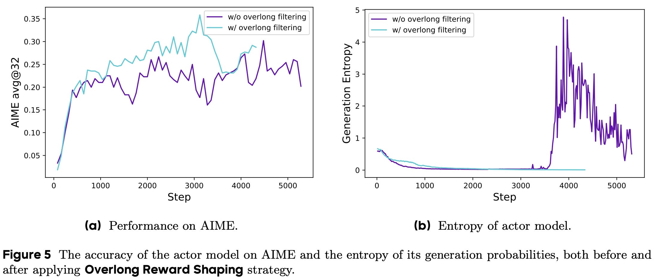
(4) Overlong reward shaping. The final improvement proposed for GRPO in [1] is related to the handling of truncated samples. During RL training, we usually impose a maximum generation length for rollouts to improve efficiency, but the policy does not always adhere to this maximum length. In some cases, the policy will attempt to generate a sample that is too long, and we will have to truncate this sample to the maximum length. The default response to this behavior in RL is punishment—we simply provide a negative reward for any truncated samples.

Interestingly, authors in [1] show that how we shape this punitive reward for truncated samples is important and can lead to training instability if handled incorrectly. For example, what if the policy’s reasoning process was totally valid but just too long? Assigning a negative reward to such a case could confuse the model. To test this theory, authors perform an experiment in which truncated samples are masked—meaning they have no contribution to the policy update—in the GRPO loss instead of being negatively reinforced. As shown in the figure below, this overlong filtering strategy improves both performance and training stability.

(from [1])

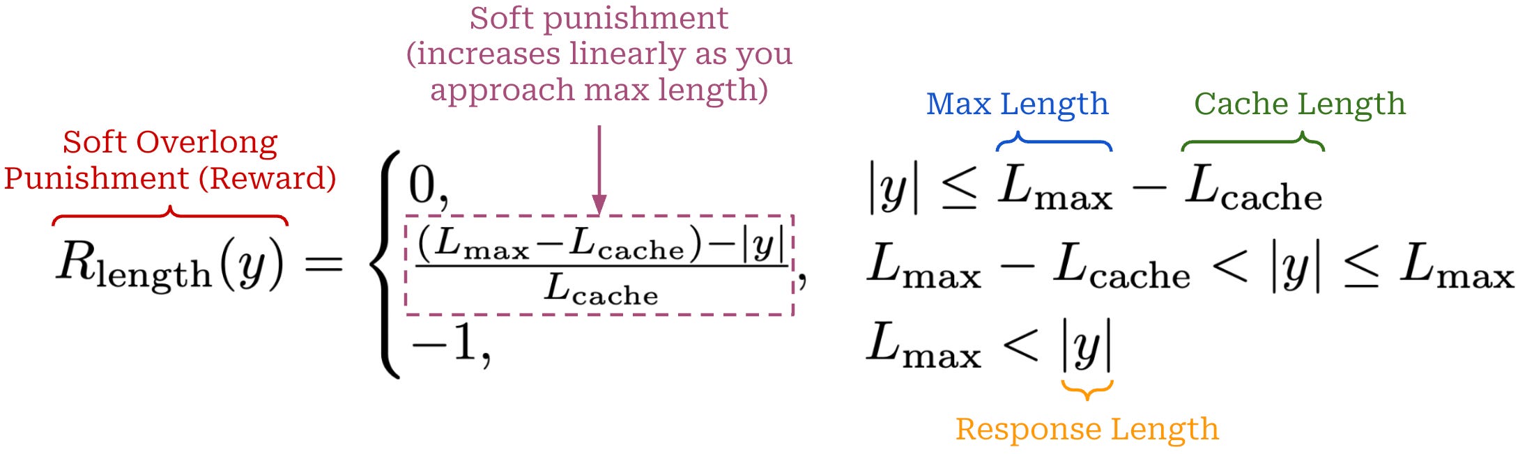
Additionally, a length-aware penalty is proposed that assigns a soft punishment to truncated samples. In particular, we define both a maximum generation length (L_max) and a cache length (L_cache), which together form the punishment interval [L_max - L_cache, L_max]. Any generation that exceeds L_max tokens in length will receive a maximum penalty of -1, while any generation less than L_max - L_cache tokens in length will have no penalty. Within the punishment interval, however, the negative reward is dynamically adjusted based on the length of the sample; see below. This soft overlong punishment is directly added to the verifiable reward in GRPO. A maximum length of 16K tokens and cache length of 4K tokens are used for DAPO experiments in [1].

Soft overlong punishment formulation (from [1])

The full DAPO algorithm, which combines the four modifications described above, is formulated by the algorithm and objective function provided below.

(from [1])

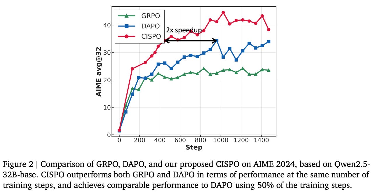
Experiments in [1] are conducted with the DAPO-Math-17K dataset⁴, which contains 17K prompts. The dataset is purposely curated so that answers are formatted as integers, making parsing and verification simple. Experiments are only performed in the math domain, but this is a common approach for evaluating algorithmic changes in RL. Due to the high cost of experimentation, researchers frequently use math RL as a testbed and assume that most findings will translate reasonably well to other domains. The Qwen-2.5-32B base model is selected to match the RL-Zero training setup of DeepSeek-R1 [2]. As shown below, accuracy on AIME increases from 0% to 50% after training with DAPO, exceeding the 47% accuracy achieved in [2].

(from [1])

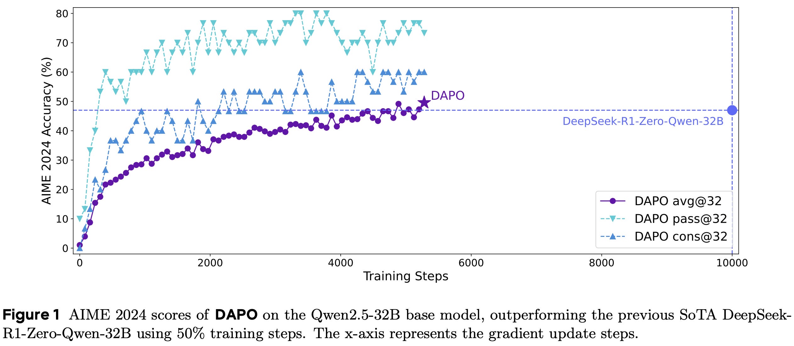
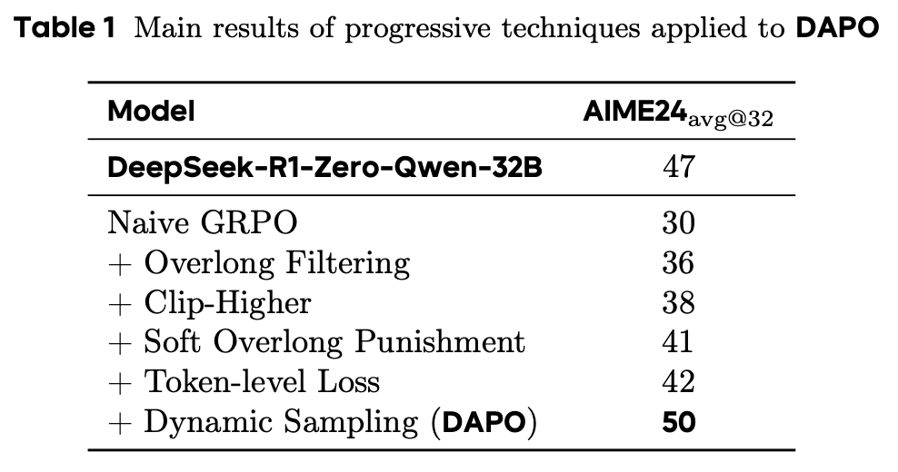
This performance is achieved using only half of the training steps required to train DeepSeek-R1-Zero-Qwen-32B, showcasing the improved sample efficiency of DAPO. In contrast, vanilla GRPO achieves an accuracy of only 30% on this benchmark. All four DAPO modifications are shown to clearly benefit final performance; see below. Although we see the smallest accuracy boost from the token-level loss, this modification makes the training process more stable. The improved health of the RL training process with DAPO is evidenced by stable increases in average response length, entropy, and training reward.

(from [1])

Understanding r1-zero-like training: A critical perspective [3]

When performing RL-Zero-style training (i.e., RL training applied directly to a base model), there are two key aspects of our training setup to consider:

1. The base model.

2. The RL training setup.

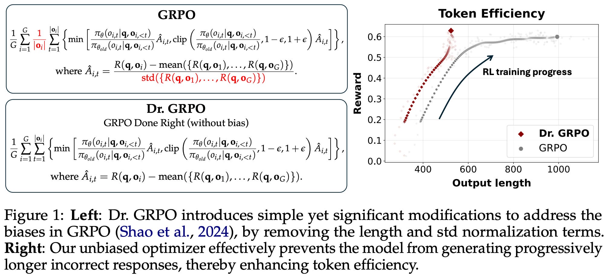
In [3], authors perform a deep investigation into these two aspects to better understand i) the impact of pretraining on performance after RL and ii) the dynamics of the RL training process in general. This investigation uncovers several interesting properties of base models that are commonly used in open RL recipes. Additionally, several biases are discovered in the GRPO loss formulation that are shown to degrade training stability and artificially inflate the length of incorrect responses. As a solution, authors propose GRPO done right (or Dr. GRPO), which uses a different advantage formulation and modified loss aggregation strategy to improve stability and address biases in GRPO.

(from [3])

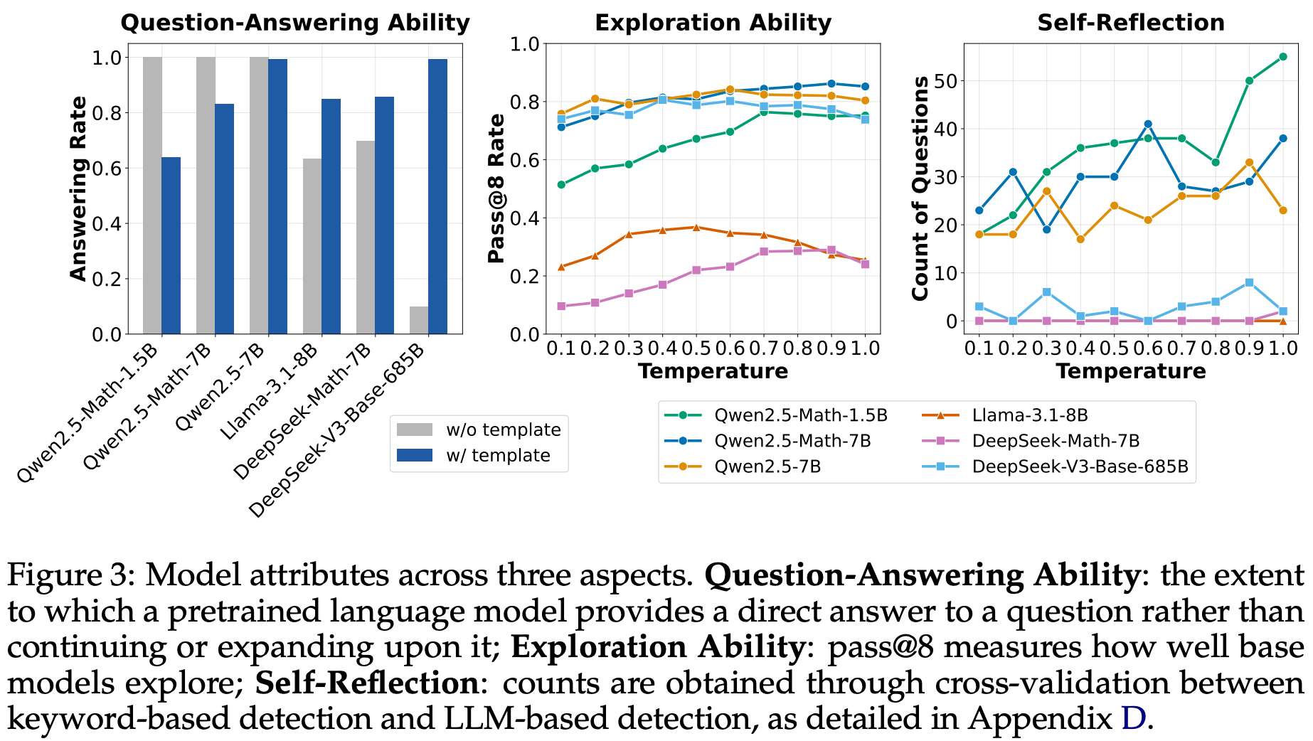
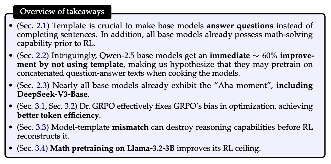
Base models. Several pretrained base models are tested in [3]—with a focus upon Qwen-2.5 (i.e., commonly used in open RL-Zero recipes) and DeepSeek-V3-Base (i.e., the original base model used for DeepSeek-R1-Zero [2])—by analyzing their responses to a set of 500 questions from MATH. The results of this analysis are summarized in the figure above and focus on two major questions:

1. Can we elicit better reasoning skills by changing the template used for prompting the base model?

2. Do base models already exhibit reasoning and self-reflection behaviors (i.e., the “Aha moment” of DeepSeek-R1) prior to RL training?

(1) Templates. Base models are trained using next token prediction and have not yet undergone any alignment. As a result, these models struggle with instruction following, making the exact template used for prompting the model important. To better understand how the selected prompt template influences base model performance, three different styles of templates are tested in [3]; see below.

(from [3])

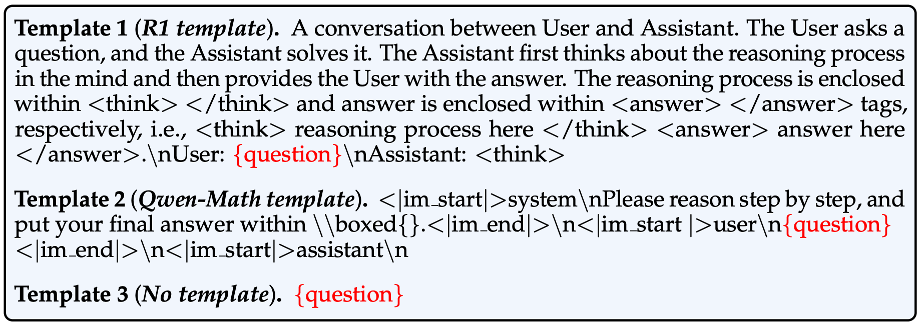
To determine the template that is most suitable for each model, GPT-4o-mini is used to assess whether questions are answered with the correct output format⁵. As shown in the figure below, the choice of template significantly influences model performance, but the most suitable template varies by model. For example, Qwen-2.5 models perform best with no template, while DeepSeek-V3 base [14] performs very poorly unless the correct chat template is used.

(from [3])

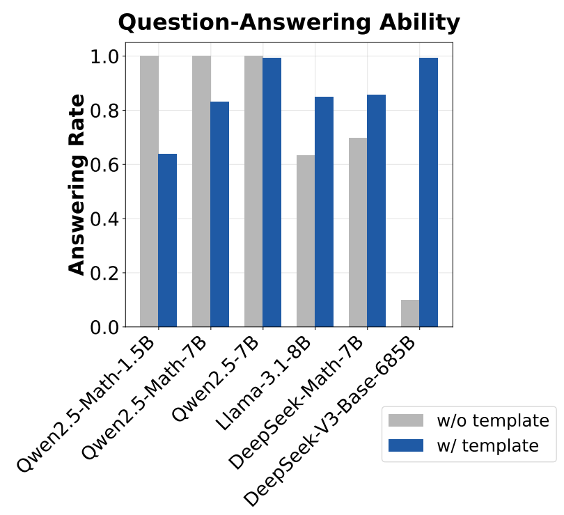
“Since Qwen2.5 uses chat model’s data (question-answer pairs) during the pretraining stage, we hypothesize that they might pretrain on the concatenated text… If our hypothesis turns out true, we shall be more careful about using Qwen2.5 models to reproduce DeepSeek-R1-Zero, since the base models are already SFT-like without templates.” - from [3]

Using a concatenated question-answer format with no template for Qwen-2.5 models leads to a 60% performance improvement, demonstrating the importance of understanding the unique properties of each base model used for RL training. In the case of Qwen-2.5, these results indicate that the base model was pretrained on concatenated question-answer data. If true, this hypothesis has significant implications for RL-Zero training—the base model has already undergone SFT-like training over question-answer pairs and thus cannot truly be considered an unaligned base model for RL-Zero-style training. However, validating this hypothesis is not possible because Qwen models do not openly disclose their training data.

Using the correct template is beneficial to the base model, but the impact is less pronounced after RL training. Similar performance is reached by most templates after RL training, despite large initial performance differences in the base model; see below. This finding hints that the performance benefits of RL may be more modest than is typically reported—model performance can be artificially deflated prior to RL training based on the exact template being used.

(from [3])

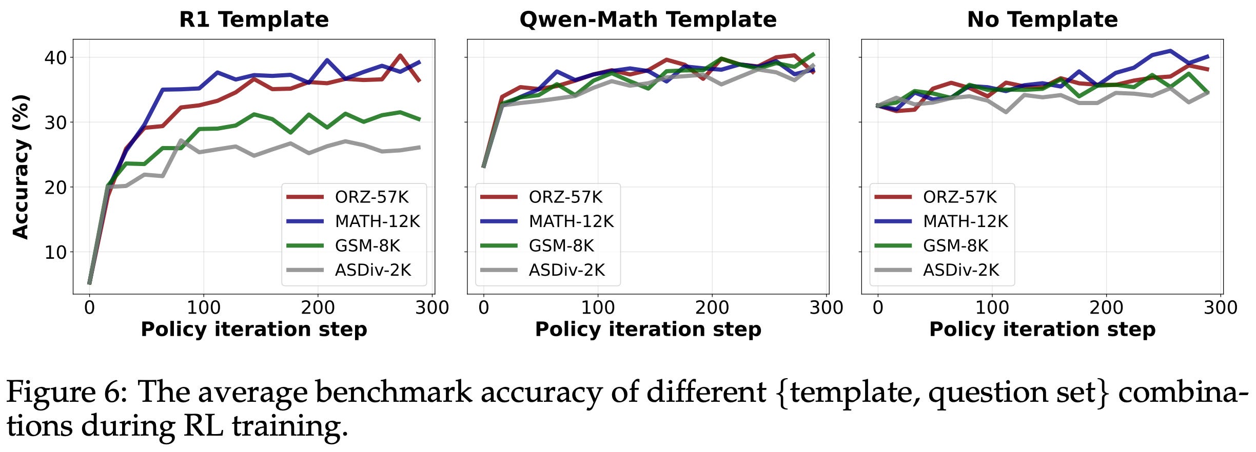
Interestingly, the ability of RL to restore full performance may depend on data coverage. More specifically, if the model and prompt template are aligned well (i.e., meaning the base model initially performs well with that prompt template), we can achieve performance benefits from RL training even on very narrow datasets (e.g., GSM-8K). However, if there is a mismatch between the base model and prompt template being used, the observed performance after RL training may suffer unless a diverse dataset with wider coverage is used; see above.

(from [3])

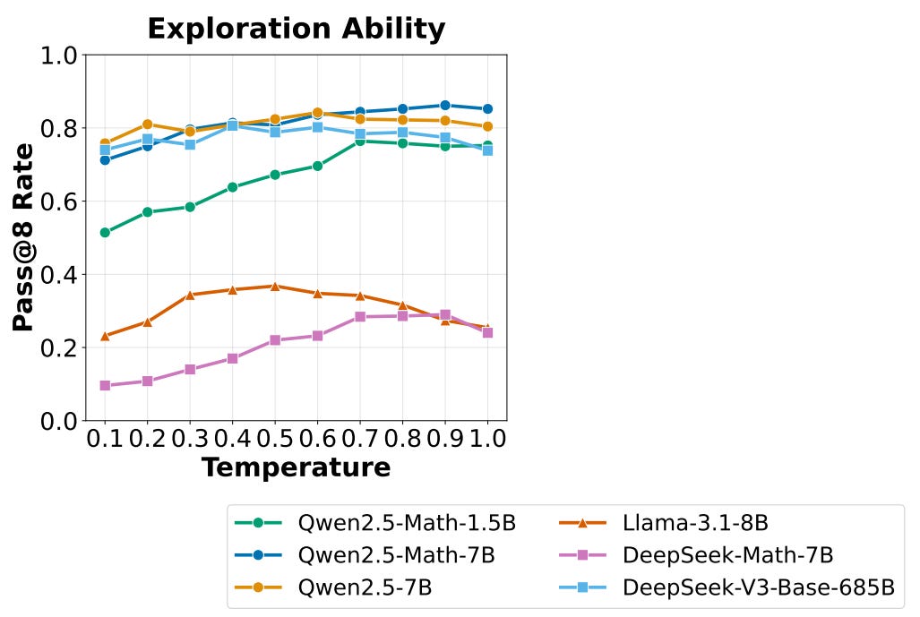
(2) Reasoning performance. After determining the most suitable template per model, authors also measure the Pass@8 performance using various temperature settings to measure base model exploration capabilities. If a base model cannot generate at least one viable solution among several rollouts, then improving reasoning capabilities with RL will be difficult—the model cannot learn to answer problems correctly via exploration. The results of this test are outlined in the figure shown above, where we see that all models have a non-zero success rate for solving reasoning problems when sampling multiple rollouts. The Qwen-2.5 and DeepSeek-V3 models already demonstrate impressive Pass@8 performance.

“If a base policy cannot even sample a single trajectory that leads to the correct final answer, it is impossible for reinforcement learning to improve the policy because there is no reward signal.” - from [3]

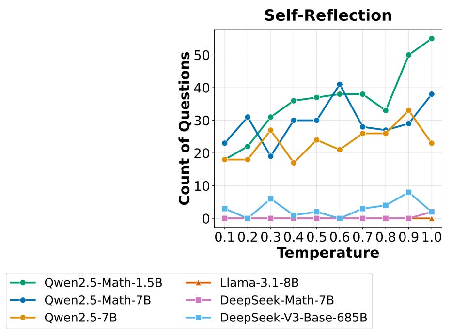
(2.5) Aha moment. The presence of an Aha moment in the RL training process of DeepSeek-R1-Zero [2] was a huge discovery in AI research, as it indicates that sophisticated reasoning behaviors can emerge naturally from RL training. However, researchers have struggled to reproduce this behavior with open models, leading many to question whether self-reflection is truly an emergent property of RL. One popular explanation for these difficulties is that base models may already exhibit self-reflection behavior prior to RL training, leading this behavior to just be emphasized—rather than completely learned—during the RL training process.

“Although self-reflection behaviors occur more frequently in R1-Zero, we observe that these behaviors are not positively correlated with higher accuracy.” - from [3]

To test this theory, authors in [3] analyze DeepSeek-V3-Base for patterns of self-reflection on the MATH dataset. This analysis reveals that the base model already uses self-reflection in a large number of queries; see below. We can find from simple keyword searches that the model outputs many “Aha” or “wait” tokens, revealing that self-reflection behavior may not be purely developed via RL. Interestingly, RL training does increase the frequency of self-reflection in the model’s output, but this behavior is not found to measurably improve performance.

(from [3])

GRPO biases. In addition to analyzing properties of base models, authors in [3] point out a few problematic biases in GRPO, as well as recommend a modified algorithm—called GRPO Done Right (or Dr. GRPO)—to fix these biases. When an LLM is trained using vanilla GRPO, we usually observe a clear increase in the model’s average response length throughout training. Such increasing response length is usually attributed to the development of long CoT reasoning abilities.

(from [3])

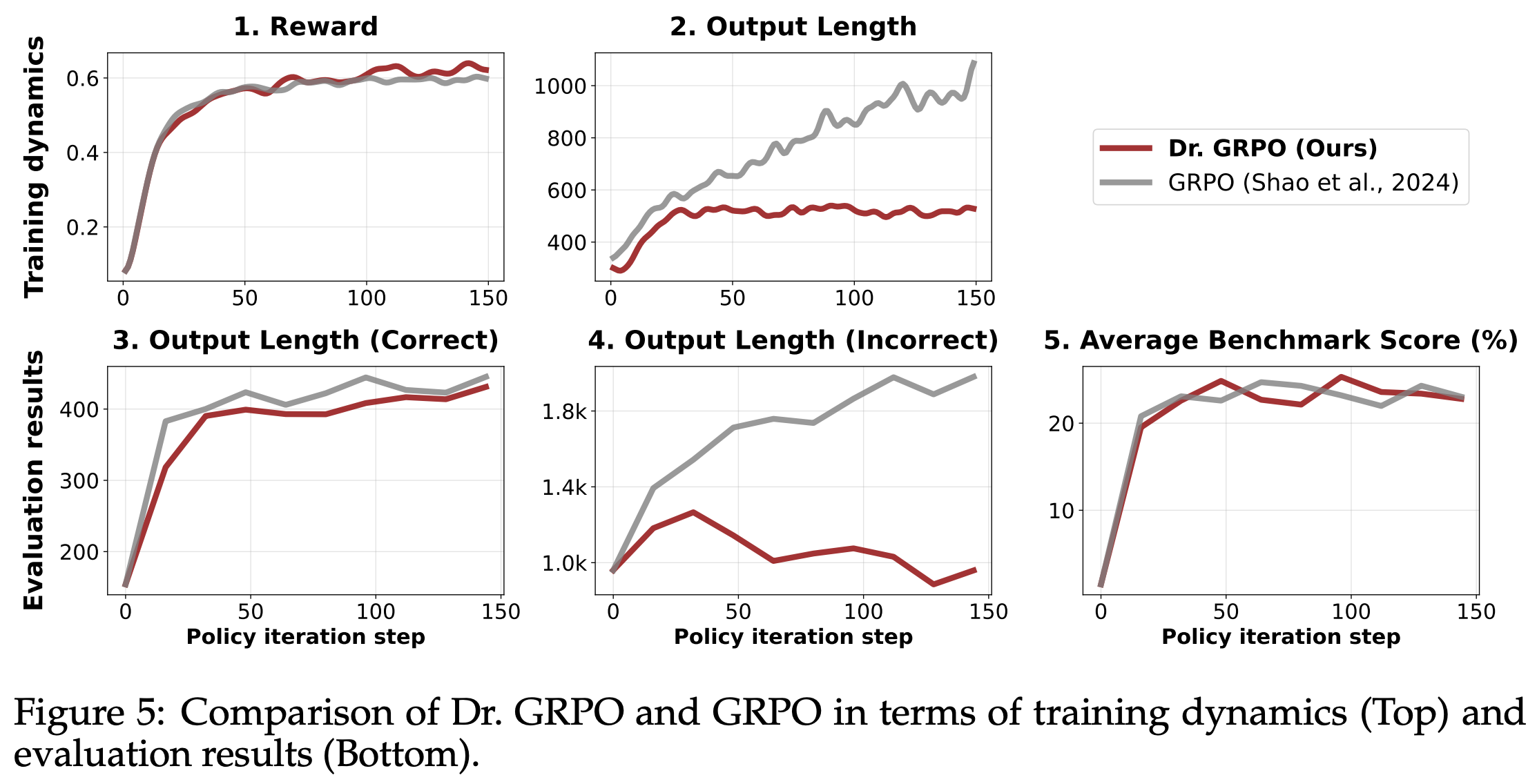
Going against common intuition for reasoning models, however, we see in [3] that this increase in response length is partially attributable to fundamental biases in the GRPO objective function. In fact, we even see in [3] that GRPO continues to increase response length after rewards begin to plateau; see above. Additionally, output lengths become noticeably longer for incorrect responses throughout the course of training, revealing a bias towards artificially inflating response lengths in GRPO. Specifically, there are two key biases that exist in the GRPO objective:

1. Response-level length bias: GRPO normalizes the summed loss of tokens in each sequence by the total number of tokens in that sequence, leading to biased gradient updates based on the length of each response.

2. Question-level difficulty biases: the standard deviation term in the denominator of the advantage formulation in GRPO causes the advantage to become very large for questions that are either too easy (i.e., most responses have a reward of one) or too hard (i.e., most responses have a reward of zero)⁶.

(from [3])

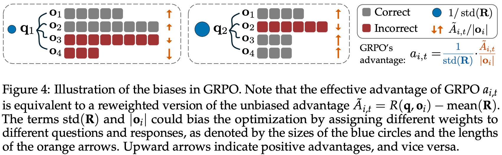
Response lengths vary during RL training, so the loss is normalized dynamically based on the length of each sequence. The response-level length bias observed in [3] matches findings in [1] that motivated the use of a token-level loss to avoid sequence lengths influencing each token’s contribution to the loss. Normalizing the GRPO loss on a sequence level leads to larger gradient updates for shorter responses—or smaller gradient updates for longer responses—when the advantage is positive. When advantage is negative, however, long responses are penalized less, leading longer responses to be preferred among incorrect outputs.

(from [3])

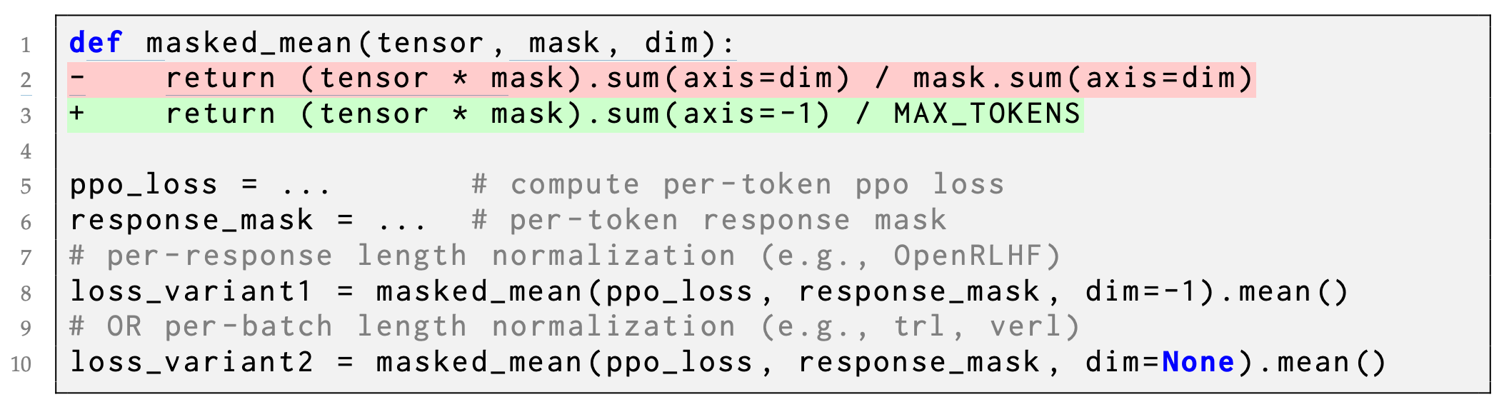
Put differently, GRPO biases the model towards overthinking by using more tokens for incorrect answers! To avoid the length bias from sequence-level aggregation, we can divide the sum of losses in each sequence by a fixed constant rather than the total number of tokens in the sequence; see above for an example implementation.

Dr. GRPO is a modified version of GRPO proposed in [3] to fix the biases outlined above. Compared to vanilla GRPO, Dr. GRPO makes two key modifications:

1. Normalizing the summed loss of each sequence by a fixed constant, rather than by the number of tokens in the sequence.

2. Removing the standard deviation term from the denominator of the advantage formulation.

Dr. GRPO is formulated below, where we see that the loss is not normalized by sequence length. The loss is instead divided by the MAX_TOKENS constant, as shown in the above code snippet. Additionally, the advantage is computed by subtracting the group-level mean of rewards from the reward for each completion (i.e., no division by standard deviation). These changes are found to mitigate the aforementioned biases and yield models that perform better on a per-token basis—better performance is achieved while outputting fewer tokens on average; see below.

(from [3])

Experiments. Dr. GRPO is implemented using the Oat framework and is released openly. Models are trained using the MATH dataset and evaluated on a variety of benchmarks, including OlympiadBench, AIME 2024, AMC, Minverva Math, and Math500. Rewards are derived based on correctness (i.e., correct responses receive a reward of one, while incorrect responses receive a reward of zero) using Math Verify. When used to train the Qwen-2.5-Math-7B model (with the Qwen-Math prompt template), the simple Dr. GRPO RL-Zero recipe achieves 43.3% accuracy on AIME 2024, which is state-of-the-art for a model of this scale; see below.

(from [3])

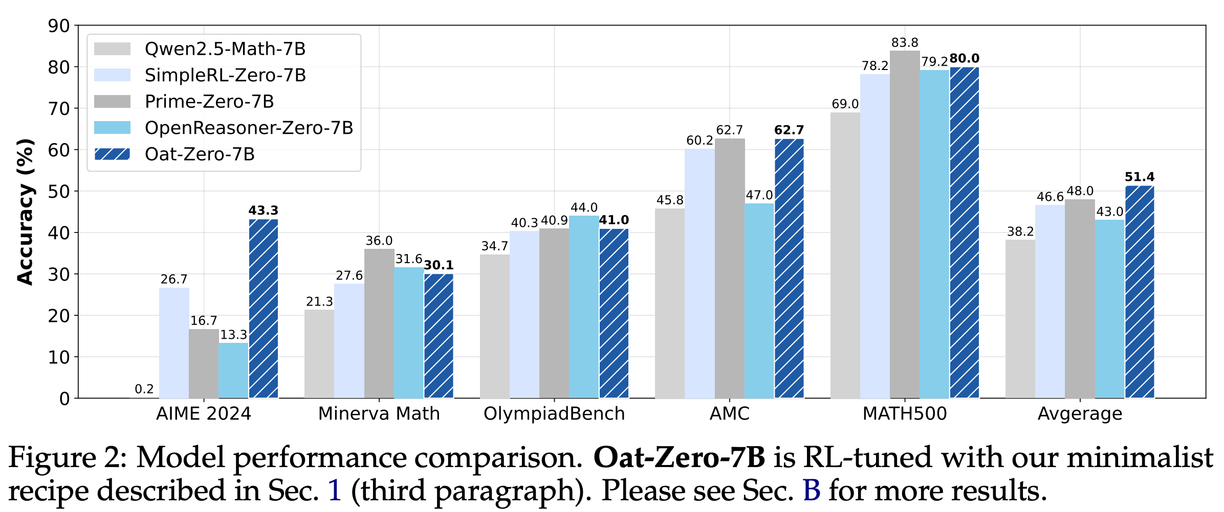
The training process for this model completes in ~27 hours on only eight A100 GPUs. Such a lightweight training setup is useful for research, as one can quickly iterate upon changes to the RL training process. The key findings from [3] are summarized in the figure below. Beyond the observed properties of base models and reported benefits of Dr. GRPO, authors in [3] find that continued, domain-specific pretraining is helpful for RL. Specifically, continually pretraining the Llama-3.2-3B model on math-specific data prior to RL-Zero training noticeably raises the model’s performance ceiling during the RL training process.

(from [3])

Your Efficient RL Framework Secretly Brings You Off-Policy RL Training [4]

During RL training, we alternate between two key operations:

1. Rollouts: given a set of prompts, sample multiple completions for each prompt using the current LLM.

2. Policy Updates: compute a weight update for the LLM using the sampled rollouts and the given objective function (e.g., from GRPO).

The cost of the RL training process is notoriously high and typically dominated by rollout generation—most of the time in RL is spent waiting for inference to finish⁷. For example, profiling the RL training process for Olmo 3 [5] reveals that 5-14× more compute is spent on inference compared to policy updates. For this reason, most modern RL training frameworks use separate engines on the backend for generating rollouts and performing policy updates. Specifically, we usually use popular training frameworks like FSDP or DeepSpeed for policy updates, while optimized inference engines like vLLM or SGLang—often with lower precision inference (e.g., int8 or fp8) for added efficiency—are used to generate rollouts.

“In modern RL training frameworks, different implementations are used for rollout generation and model training… We show the implementation gap implicitly turns the on-policy RL to be off-policy.” - from [4]

For simplicity, we will refer to the engines used for sampling rollouts and computing policy updates as the sampler and learner engines, respectively.

Gap between engines. One may naively assume that engine implementations should be similar, but the use of separate sampler and learner engines creates a mismatch in the code used for rollouts and policy updates. Even when engines share the same exact model parameters, the token probabilities that they predict can differ significantly; see below. In the worst case, token probabilities are completely contradictory between the two engines, meaning that the learner would not have generated the same completion as the sampler. In this case, the RL training process actually becomes off-policy, thus degrading performance.

Difference in token probabilities created by the mismatch between sampler and learner engines (from [4])

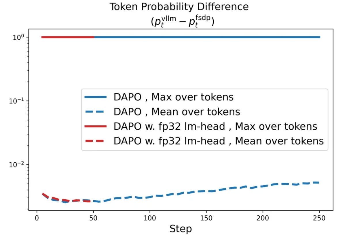
We must address this implementation gap for RL training to be truly on-policy. To accomplish this, we could (obviously) take an engineering-centric approach—just find and eliminate implementation differences so that the two engines yield identical token probabilities. In [4], authors take this approach by identifying problem areas that contribute to differences in token probabilities, but the implementation gap still exists even after patching several issues in the engine code; see above.

To fully eliminate this implementation gap, we must chase down an even larger number of subtle issues that exist, such as precision differences throughout parts of the model or deviations in sampling code. Identifying and removing all of these bugs is a tedious engineering process that must be repeated any time a new (or even slightly modified) engine is used for RL. Going further, even if all of these issues are addressed, the LLM inference process is still fundamentally non-deterministic. As a result, the engine gap can be minimized but not fully removed. For these reasons, an engineering-centric solution, though conceptually simple, is resource-intensive and difficult to achieve in practice.

Importance Sampling. Authors in [4] propose an algorithmic approach based on importance sampling for addressing the engine mismatch in RL. Formally, importance sampling is a statistical method used to estimate properties (e.g., an expectation) of a target probability distribution f(x) by sampling from a proposal distribution g(x). Usually, sampling from g(x) is much cheaper than sampling from f(x), which is the motivation for importance sampling.

(source)

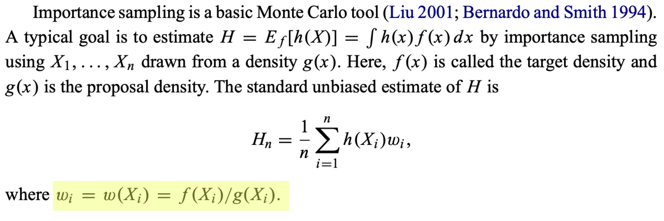
In other words, if sampling from f(x) is difficult, we can instead choose to draw samples from g(x) and just correct for the discrepancy between f(x) and g(x) by weighting each sample by the importance ratio f(x) / g(x); see above. This concept can be directly applied in the context of RL! Namely, we can denote the token probabilities from our learner and sampler as f(x) and g(x), respectively. From our prior discussion, we know that:

1. Sampling from g(x) is much more efficient relative to f(x).

2. There is a discrepancy between these two distributions.

Therefore, importance sampling can be directly used to correct for this mismatch.

“When direct Monte Carlo estimation of the expected value under a target distribution is difficult, importance sampling allows us to sample from an alternative distribution instead. In our case, the target distribution is π_learner, but it is extremely slow to sample from. Using a separate backend (e.g., vLLM) for rollout generation means that we are sampling from π_sampler instead. The discrepancy is then corrected by weighting each sample with an importance ratio.” - from [4]

Truncated Importance Sampling (TIS) for RL. To understand how importance sampling can be practically implemented in the context of RL training, let’s begin with the most basic expression for a policy gradient; see below.

Basic policy gradient expression

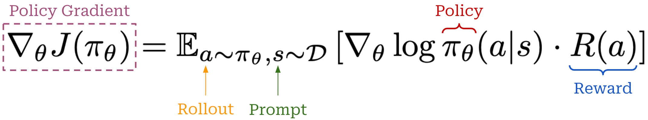
In practice, the policy gradient that we can compute looks slightly different from this, as we are not using the same policy for sampling the rollout and computing the policy gradient. Rather, the actual expression we will use is shown below, where separate engines are used for the rollouts and policy gradient.

Basic policy gradient expression with different engines and TIS

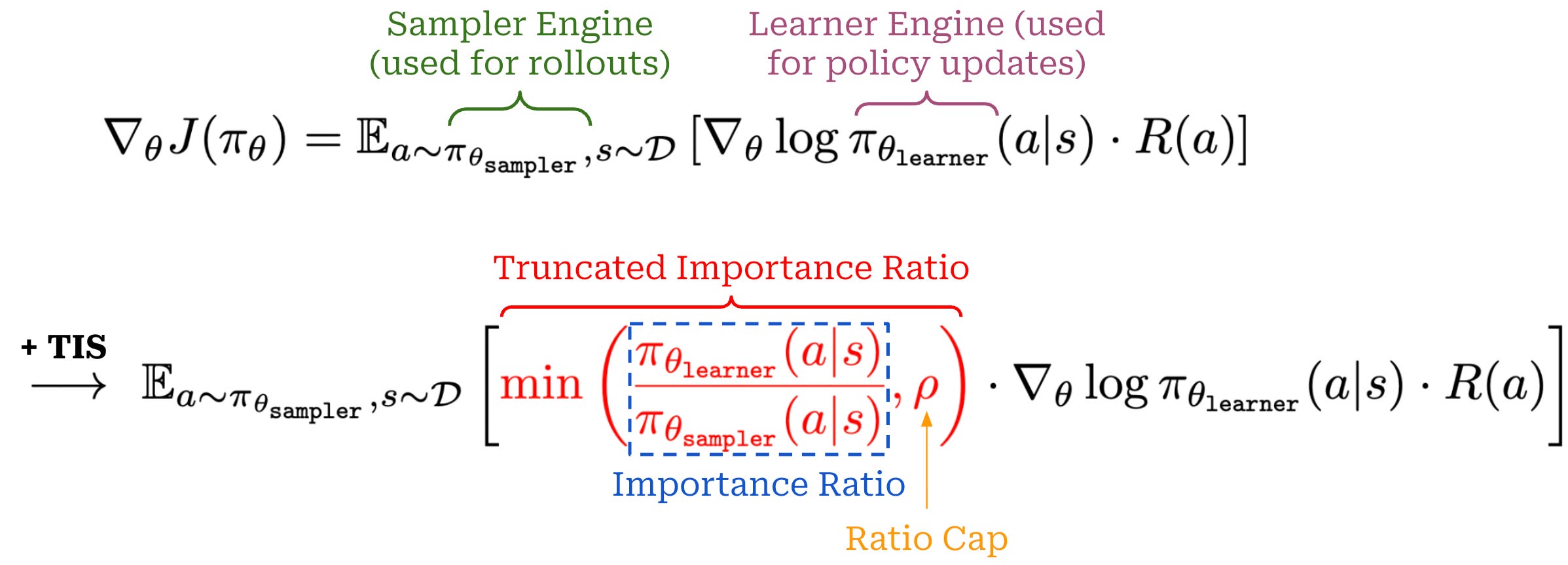
As shown above, importance sampling operates by weighting the policy gradient by the importance ratio f(x) / g(x). For RL training, the importance ratio is computed as π_learner / π_sampler (i.e., the ratio of token probabilities from the learner and sampler engines). To make the policy update more stable, authors in [4] adopt truncated importance sampling (TIS), which simply caps the importance ratio at a maximum value of ρ. The policy gradient is not changed much—we just scale the gradient expression by the (truncated) importance ratio.

“While there has been extensive study on how to design a stable and effective importance sampling, in practice we find it usually sufficient to use a classical technique, truncated importance sampling.” - from [4]

We formulate TIS with a basic policy gradient expression above, but extending this idea to other RL optimizers is straightforward. In particular, we can just:

• Take the policy gradient expression for our RL optimizer of choice.

• Scale the new policy gradient expression by the same importance ratio.

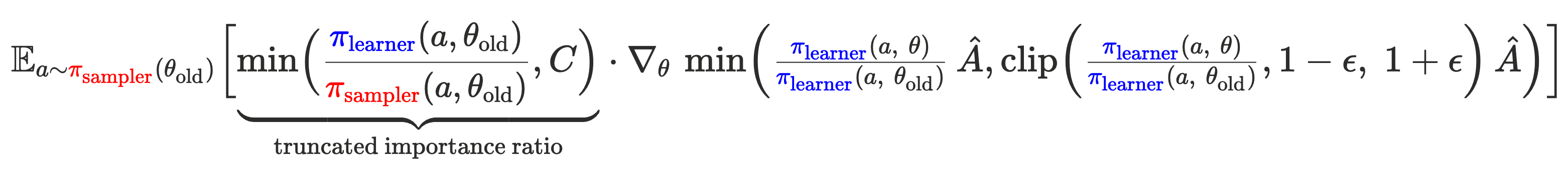
For example, we can apply TIS to GRPO or PPO as shown below⁸. After computing the policy gradient, we can multiply this gradient by the (truncated) importance ratio. We still scale the policy gradient by the importance ratio, but we substitute our standard policy gradient expression with that of GRPO.

Policy gradient with TIS for GRPO or PPO (from [4])

Does TIS work? To determine whether TIS solves the mismatch problem, authors in [4] first conduct experiments using Qwen-2.5-32B with DAPO [1] on the DAPO-Math-17K dataset. Due to resource limitations, RL training is stopped after 250 iterations, but these initial iterations can be used to analyze the properties of the training process. An early stopping approach is commonly used to efficiently test interventions to the RL training process. As shown below, we see a clear boost in performance when TIS is used in DAPO—TIS benefits performance significantly. Additionally, we see that similar performance cannot be achieved by addressing implementation gaps between engines (i.e., an engineering-centric approach).

(from [4])

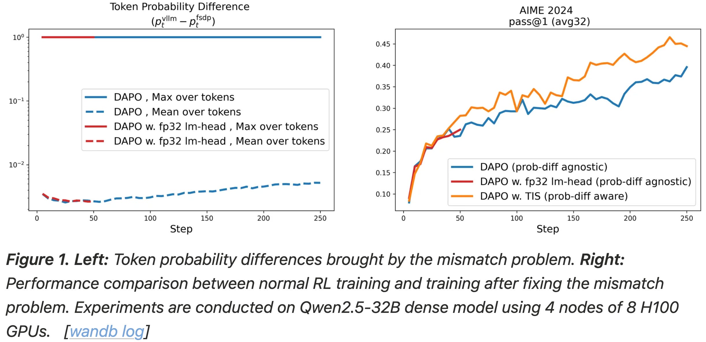
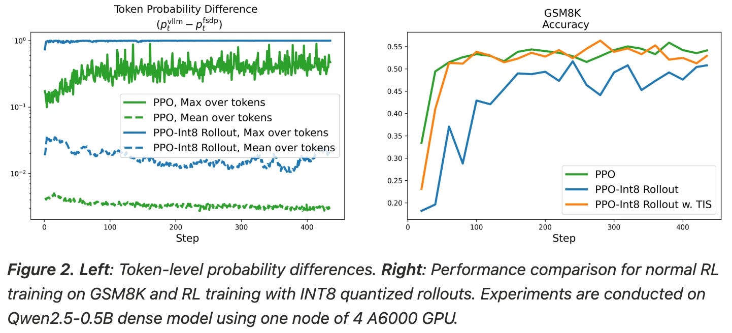
Quantized rollouts, which refers to sampling rollouts in a lower numerical precision (e.g., fp8 or int8 instead of bf16), can be used to study the impact of the distribution gap between sampler and learner engines. We can increase this gap by lowering the precision used for generating rollouts. To test the impact of increasing the mismatch in this way, a basic GSM8K setup is used in [4], where rollouts are sampled using either bf16 or int8 precision.

Using lower precision is shown in [4] to increase the maximum difference in token probabilities from ~0.4 to ~1.0, thus confirming that quantized rollouts do measurably increase the gap between the sampler and learner. As shown below, performing regular PPO training with quantized rollouts results in noticeable performance deterioration. By using TIS, we can mitigate this issue and match the performance of the higher precision (bf16) training setup; see below.

(from [4])

Analyzing the impact of quantized rollouts further, we see in [4] that experiments using int8 rollouts i) show clear signs of entropy collapse and ii) produce models with abnormally long average response lengths. Both observations indicate poor health in the RL training process. Entropy collapse is not observed when using bf16 rollouts, revealing that the RL training process is negatively impacted by the mismatch introduced by quantized rollouts. However, using TIS is also found to effectively address the mismatch and reverse these observations; see below.

(from [4])

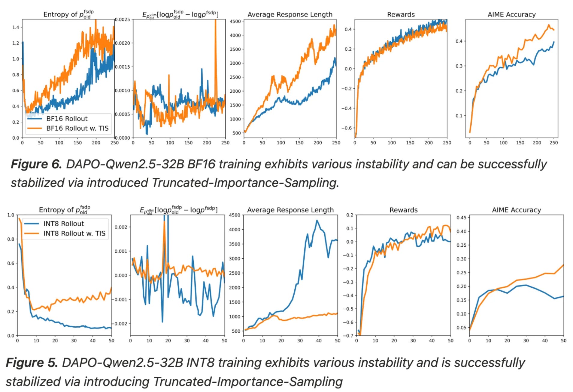
Although the bf16 training setup is already stable, using TIS even with bf16 rollouts is found to further improve entropy values, which can allow the model to explore more during RL; see above. Generally, TIS should not provide much of a benefit when the mismatch between sampler and learner engines is small—the importance ratio in these cases is ~1.0 and the objective becomes identical to standard PPO or GRPO. However, TIS does not deteriorate performance in these cases and can still yield some benefits, as shown in the case with bf16 rollouts.

What causes the gap? To conclude their analysis, authors in [4] study practical choices that can worsen the sampler-learner gap in RL. To quantify the size of the gap, token-level probability mismatch is measured per response—either using the mean or maximum difference across tokens in the response—over a set of 512 prompts from DAPO-Math-17K. From this analysis, we learn that:

• Mean mismatch tends to stay the same between most implementations—the largest impact is observed in terms of maximum mismatch. In other words, large sampler-learner gaps are characterized by a noticeable increase in the maximum token probability discrepancy across sequences.

• Differences in parallelism strategies significantly increase the mismatch (e.g., sequence parallelism in the learner and tensor parallelism in the sampler).

• Using the same parallelism strategy with different settings (e.g., tensor parallelism with 2 versus 4 GPUs) is less problematic compared to using different distribution strategies altogether.

• Using longer rollouts in RL tends to increase the sampler-learned gap.

• Using different sampler backends (e.g., vLLM, SGLang, or SGLang with deterministic kernel) does not impact the sampler-learner gap.

“Responses capped at 20K tokens exhibit a higher maximum mismatch than those capped at 4K… the mean mismatch remains similar across both settings… longer sequences provide more opportunities for a single, large probability divergence, even when the average per-token difference remains stable.” - from [4]

Beyond the factors mentioned above, there are other choices that may impact the sampler-learner gap but are not deeply analyzed in [4]. For example, dense models exhibit different levels of mismatch compared to Mixture-of-Experts (MoE) models, while base models tend to have a smaller mismatch compared to models that have already been post-trained. Additionally, the mismatch can fluctuate depending upon characteristics of our data (e.g., difficulty or domain).

More Tweaks: GSPO, GMPO, CISPO and Beyond

We have now learned about the most popular GRPO modifications that have been recently proposed, but there are still many other useful papers in this space. This section will provide a wider overview of such work with links to further reading.

“Unlike previous algorithms that adopt token-level importance ratios, GSPO defines the importance ratio based on sequence likelihood and performs sequence-level clipping, rewarding, and optimization.” - from [6]

Group Sequence Policy Optimization (GSPO) [6] is a modified version of GRPO that yields benefits in terms of stability and efficiency, especially for MoE models. The GSPO algorithm was used for training Qwen 3 models, which are (at the time of writing) the most performant and widely used open weight models. The key idea behind GSPO is changing the loss to operate at the sequence level instead of the token level. Most LLMs are trained using outcome rewards, meaning the reward is assigned at the sequence level. Assuming a single outcome reward, GRPO assigns the same advantage to every token in a sequence. Despite using outcome supervision, however, the surrogate loss in GRPO defines a per-token policy (or importance) ratio that scales the gradient of each token; see below.

Token-level importance and sequence-level advantage in the GRPO loss

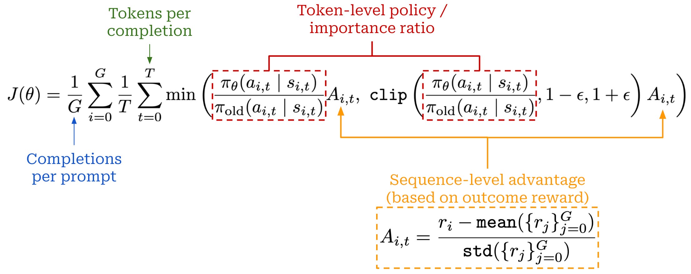
In this standard formulation of the surrogate objective in GRPO, there is a misalignment between how the model is optimized—on the token level—and how rewards are assigned—on the sequence level. Using token-level importance ratios increases the variance of the policy gradient and can lead to training stability issues in large-scale RL runs. To avoid these issues, GSPO instead computes the importance ratio on the sequence-level, which aligns naturally with the reward structure used for LLMs and improves training stability; see below.

GSPO loss function (from [6])

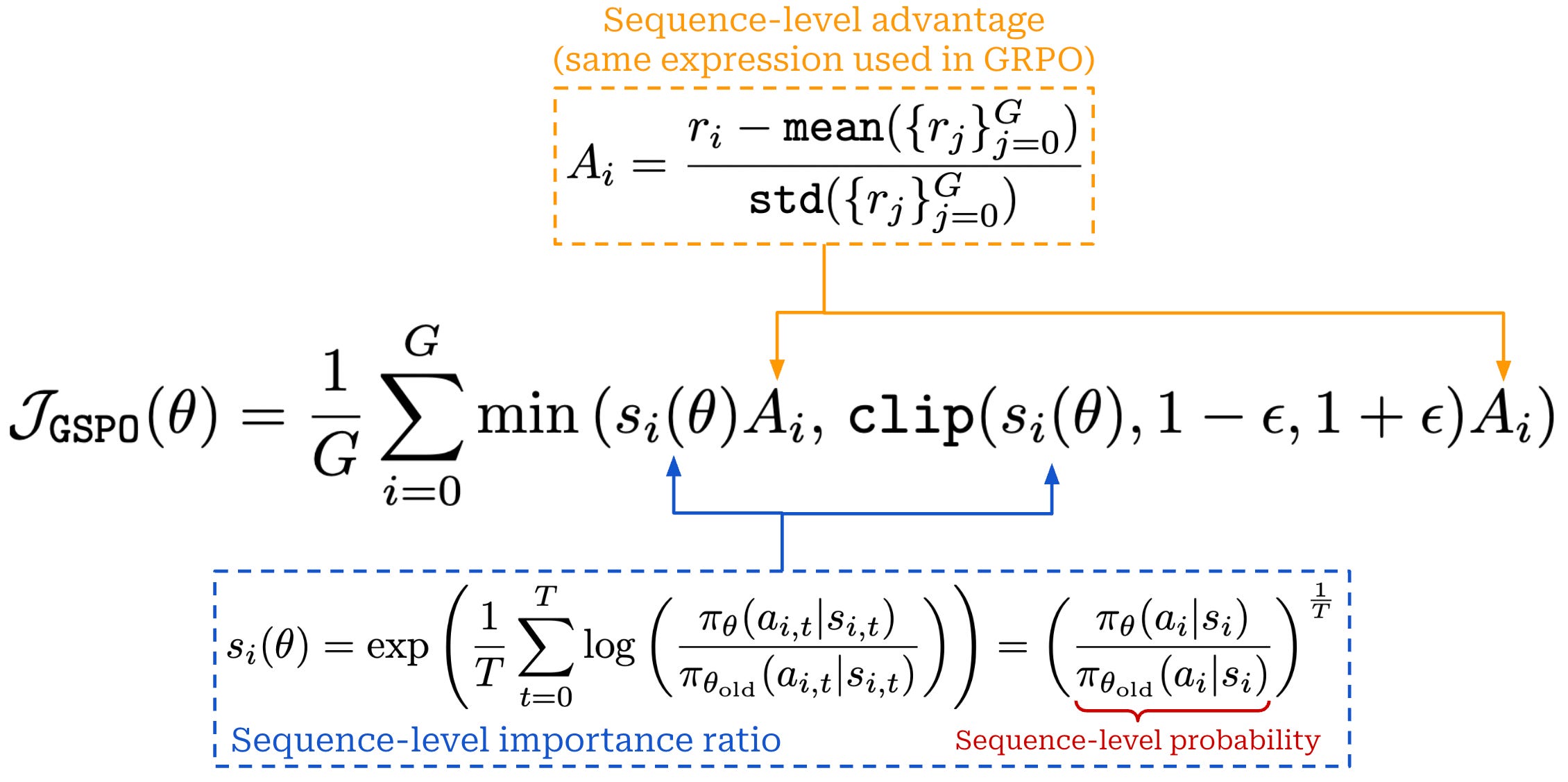
The importance ratio is computed using the probability of the entire sequence, and we apply clipping to this sequence-level importance ratio. By doing this, we apply a stable sequence-level weight to all tokens, rather than introducing token-level importance weights with high variance. Notably, the importance ratio in GSPO is still normalized by the number of tokens in a completion T, ensuring that the ratio does not fluctuate drastically based on the length of a sequence. GSPO also uses the same advantage formulation as GRPO, allowing it to keep the same computational efficiency (i.e., from not using a value model).

(from [6])

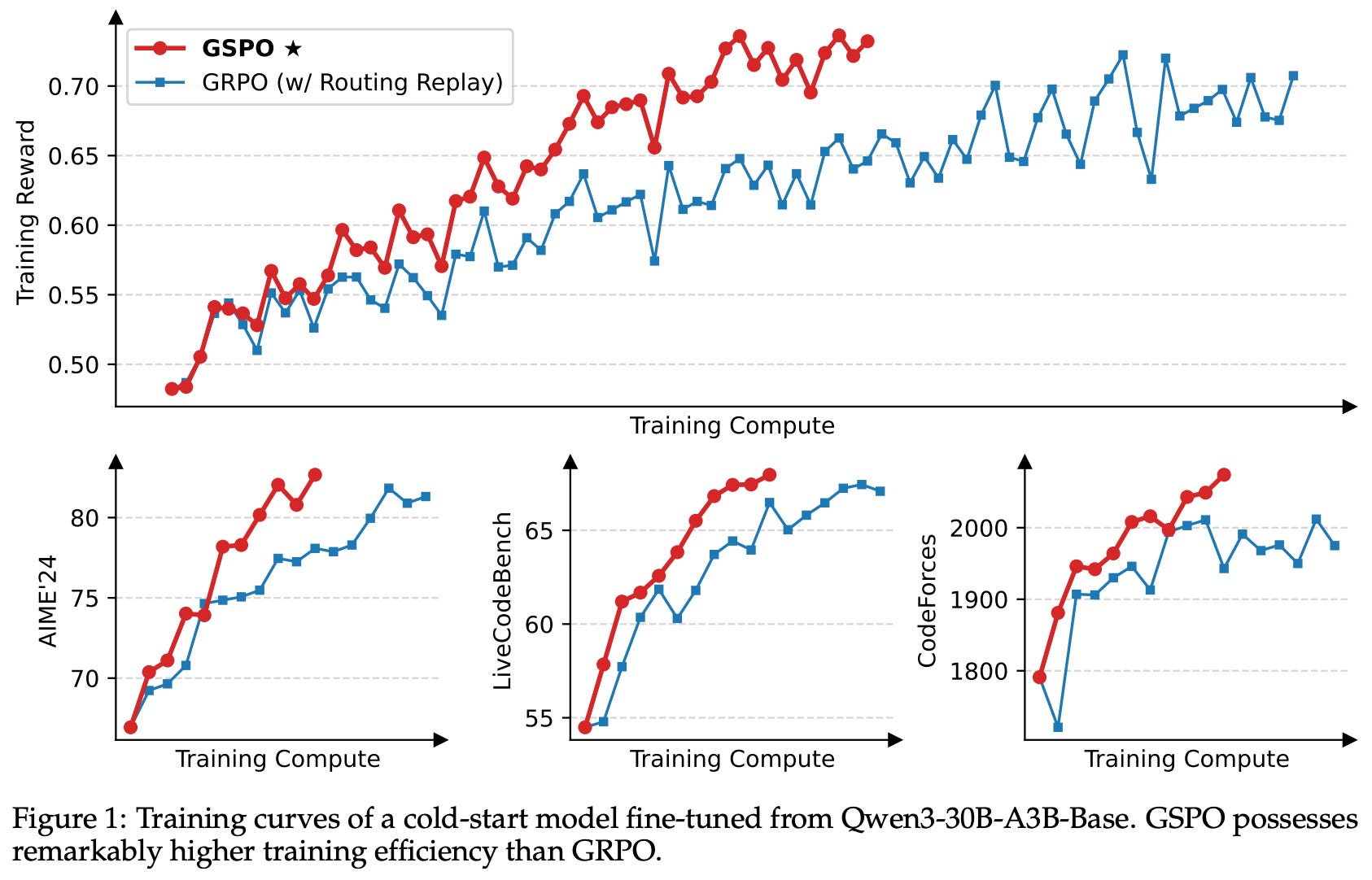
When used in experiments, GSPO not only improves training stability, but also offers better sample efficiency and overall performance; see above. The stability of GSPO is found to be especially useful when training large MoE models, such as Qwen3-235B-A22B. In particular, we often experience expert-activation volatility when training MoEs with RL, meaning that a large portion of experts active for a given prompt change or fluctuate drastically after one or more policy updates. This volatility in expert selection can prevent convergence during RL training.

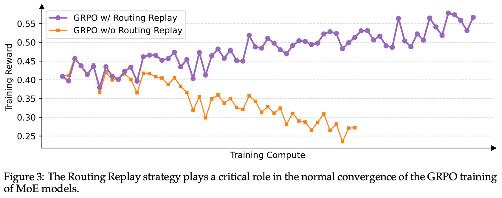
Initially, Qwen 3 models solved this issue via routing replay, which caches the initial experts selected for a prompt and uses these same experts for computing several subsequent policy updates. Routing replay enables convergence of MoE models when trained with GRPO. However, GSPO naturally provides stable RL training for MoEs without the need for any complex workarounds; see below.

(from [1])

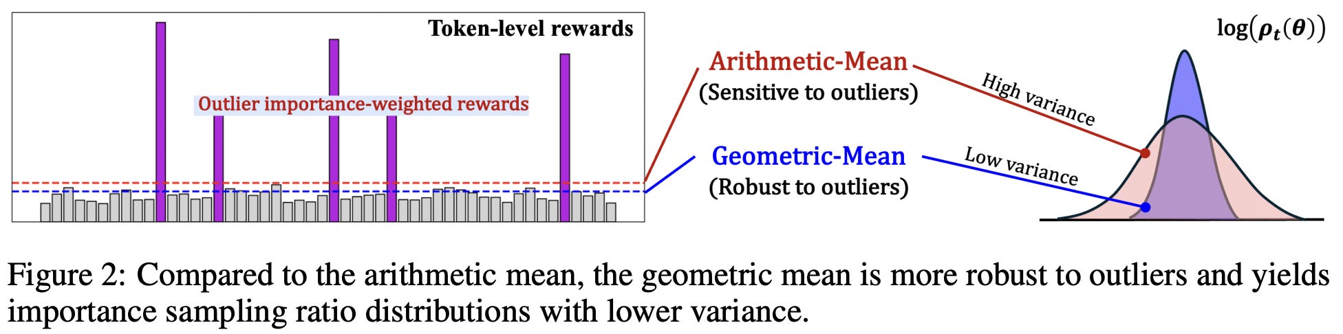
Geometric Mean Policy Optimization (GMPO) [7] addresses the same problem observed by GSPO but uses a different approach. During RL training with GRPO, token-level importance ratios can become large in magnitude, creating outlier importance weights that cause training instability. GMPO solves this issue by using a new aggregation strategy for the loss. In GRPO, the loss is aggregated by taking the mean of token-level losses over the sequence. GSPO improves stability by calculating importance ratios at a sequence level (i.e., not the token level). In contrast, GMPO still uses token-level importance ratios, but we aggregate the token-level loss by taking a geometric mean over the sequence; see below.

(from [7])

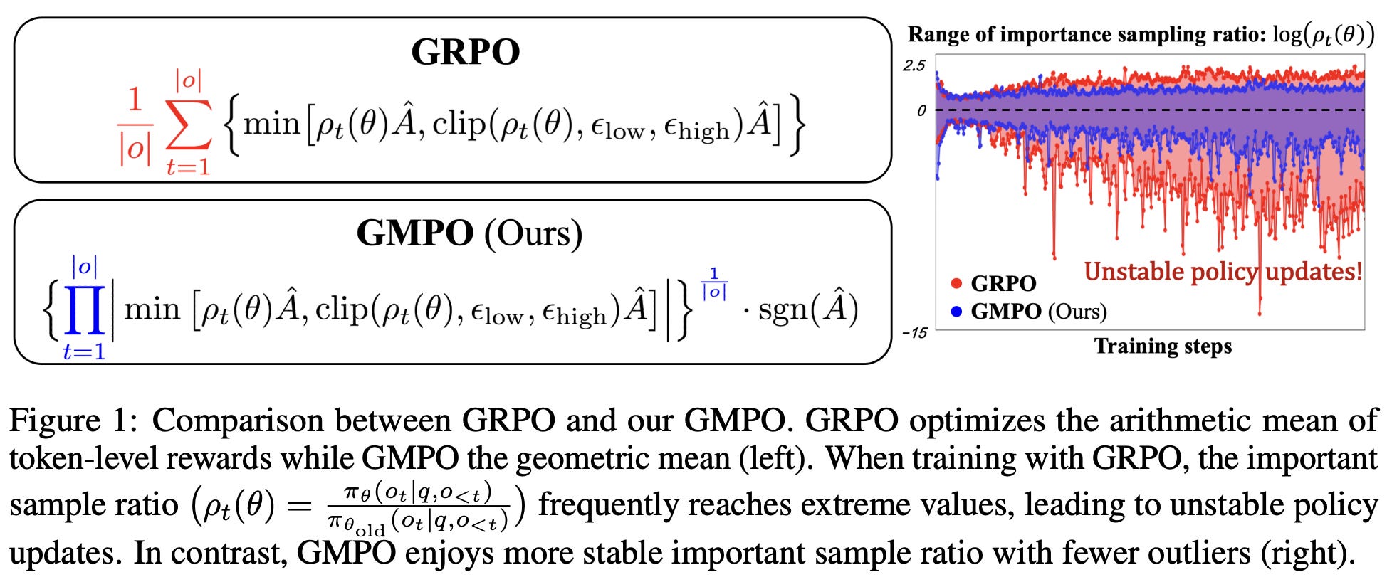
Because geometric means involve taking roots, they are only defined for non-negative numbers. To get around this, the geometric mean in GMPO is computed over absolute values of token-level losses and multiplied by the sign of the advantage (i.e., either -1 or 1) to ensure correct directionality of the update.

“GMPO is plug-and-play—simply replacing GRPO’s arithmetic mean with the geometric mean of token-level rewards, as the latter is inherently less sensitive to outliers.” - from [7]

Given that arithmetic means are sensitive to outliers, outlier importance ratios during RL training can cause instability in the standard GRPO loss. On the other hand, geometric means are less sensitive to outliers and can, therefore, help to reduce the variance of the policy gradient; see below.

(from [7])

Although GMPO still uses token-level importance ratios and applies clipping at the token level, a wider clipping range is needed relative to GRPO; e.g., authors in [7] use a range of [~0.7, ~1.5] instead of the default [0.8, 1.2] range used by GRPO. To ensure numerical stability, we usually compute importance ratios (and the entire geometric mean) using log probabilities instead of raw probability values. See below for an example—this is a common practical trick used by most PPO-style algorithms⁹. The clipping range used for GMPO corresponds to clipping the log of the importance ratio within the range [-0.4, 0.4].

Example implementation of the GMPO loss (from [7])

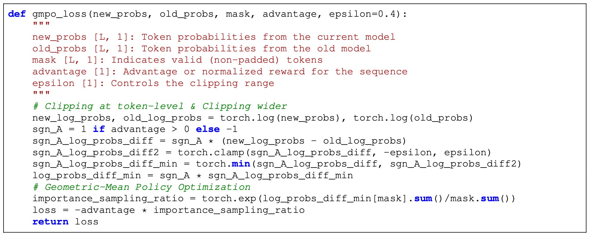
We learn from ablations in [7] that token-level clipping outperforms computing and clipping importance ratios at the sequence level. Importance ratios during RL training lie in a more stable range relative to GRPO as well; see below.

(from [7])

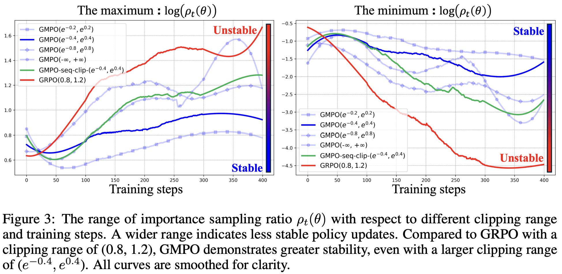
Compared to GRPO, GMPO also has more stable entropy during training, which is a positive sign of exploration. In the math domain, GMPO improves Pass@1 performance by as much as 4% absolute, and the largest performance benefits are observed when training multimodal and MoE models.

Clipped Importance Sampling Weight Policy Optimization (CISPO) [8] is a modified variant of GRPO that is proposed in the MiniMax-M1 technical report and shown to benefit training stability in experiments with large-scale RL. In experiments with PPO and GRPO, authors in [8] observe that “fork” tokens in the model’s reasoning trace (e.g., “aha” or “wait”) are rare and tend to have low probabilities, leading them to be assigned large importance ratios. Unfortunately, these pivotal fork tokens, which play an important role in the LLM’s reasoning process and help to stabilize entropy during training, are usually clipped by the GRPO objective, which eliminates their contribution to the policy update.

“We found that tokens associated with reflective behaviors… were typically rare and assigned low probabilities by our base model. During policy updates, these tokens were likely to exhibit high [importance ratio] values. As a result, these tokens were clipped out after the first on-policy update, preventing them from contributing to subsequent off-policy gradient updates… These low-probability tokens are often crucial for stabilizing entropy and facilitating scalable RL.” - from [8]

In DAPO [1], this issue is addressed via the clip higher approach, which lessens restrictions on policy updates for exploration tokens by increasing the upper bound of clipping in GRPO. However, such an approach is less effective for MiniMax-M1 because 16 policy updates are performed over each batch of data—most standard RL setups perform fewer (~2-4) updates. Usually, the importance ratio will exceed the clipping range after a few policy updates, and tokens with larger ratios will eventually be ignored by all subsequent policy updates. Ideally, we should allow pivotal exploration tokens to contribute to all policy updates.

CISPO uses the same advantage estimation technique as GRPO, but the structure of the objective resembles that of REINFORCE; see below. Unlike REINFORCE, however, token-level losses in CISPO are scaled by a clipped version of the importance ratio. Due to the use of a stop gradient, the importance ratio is treated as a constant that scales each token’s contribution to the overall policy gradient, but it is not backpropagated when computing the gradient.

CISPO loss (from [8])

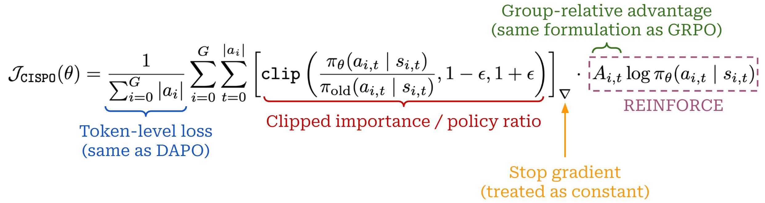
For PPO and GRPO, tokens that are clipped from the loss receive zero gradient—they have no contribution to the policy update. By treating the importance ratio as a capped constant, CISPO adopts a soft, token-level clipping strategy. Clipped tokens still contribute to the gradient, but their weight is capped at a maximum value, as determined by the clipping mechanism in CISPO. When compared to GRPO and DAPO [1] for training Qwen2.5-32B-Base on math reasoning tasks, CISPO is found to improve both stability and sample efficiency; see below.

(from [8])

More GRPO variants. Given the popularity of reasoning and RL in current LLM research, there are many modified algorithms and practical tweaks that have been proposed in the wake of GRPO. Only a small (though notable!) part of this work has been covered in this overview. To learn more, there are several great posts beyond this overview that have been written on the topic. Additionally, a list of other notable works in the area has been compiled below:

• Router-Shift Policy Optimization (RSPO) is an MoE-focused RL algorithm that rescales router logits to improve training stability.

• Soft Adaptive Policy Optimization (SAPO) replaces clipping for the policy ratio with a softer gating mechanism to encourage stable policy updates.

• Low-Probability Token Isolation (Lopti) reduces the effect of low-probability tokens on the policy gradient and emphasizes parameter updates driven by high-probability tokens to improve the efficiency of RL.

• Value-based Augmented Proximal Policy Optimization (VAPO) builds upon work in DAPO to improve RL efficiency via the introduction of value models.

• Lite PPO performs an extensive empirical analysis of RL for reasoning, arriving at a critic-free RL algorithm—based upon the vanilla PPO loss—that consistently outperforms GRPO and DAPO. The main idea is to perform token-level loss aggregation and compute the standard deviation from the GRPO advantage over the entire batch instead of the group.

• Dynamic Clipping Policy Optimization (DCPO) proposes a dynamic clipping scheme for token-level importance ratios and standardizes rewards across consecutive training steps to avoid cases with zero policy gradients.

• Reinforce-Rej proposes a simple scheme—inspired by rejection sampling—that improves RL efficiency by removing entirely correct and incorrect samples during training (similarly to dynamic sampling).

If you are aware of any other works that propose improvements to GRPO, please share them in the comments so that this list can be improved and expanded!

Putting It All Together

“Our TIS fix addresses the distribution mismatch problem rooted in the system level… Such a problem widely exists in RL training frameworks… our fix can be applied irrespective of the specific RL algorithms used.” - from [4]

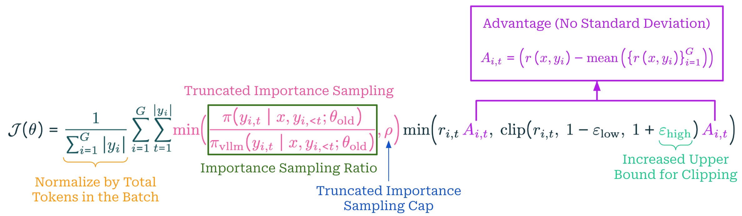
Throughout the course of this overview, we have seen a wide variety of tips and tricks that can be applied to improve the effectiveness of RL training with GRPO. Despite the breadth of this work, we must remember that these proposals are not mutually exclusive—the most performant RL setups will combine many best practices together. For example, Olmo 3 [5] provides a perfect example of an RL training pipeline that incorporates several techniques from recent research. Specifically, the following set of improvements are adopted for training the Olmo 3 Think reasoning models with GRPO:

• Zero Gradient Filtering: prompts for which the entire group of completions or rollouts in GRPO receive the same reward are removed [1].

• Active Sampling: to maintain a constant batch size despite filtering zero-gradient examples, additional samples are always available to replace those that are filtered out [1].

• Token-Level Loss: the GRPO loss is normalized by the total number of tokens across the batch instead of per-sequence, which avoids instilling a length bias in the loss [1].

• No KL Loss: the KL divergence term is removed from the GRPO loss to allow for more flexibility in the policy updates, which is a common choice in recent reasoning research.

• Clipping Upper Bound: the upper bound in the PPO-style clipping used by GRPO is set higher than the lower bound to enable larger policy updates [1].

• Truncated Importance Sampling (TIS): an extra importance sampling term is added to the GRPO loss to adjust for differences in log probabilities between engines used for training and inference [4].

• No Standard Deviation: the standard deviation of rewards in a group is excluded from the denominator of the GRPO advantage calculation [3].

The modified GRPO objective for Olmo 3 is shown below. Compared to vanilla GRPO, we maintain the high-level structure of the loss but i) normalize the objective differently, ii) slightly change the advantage, iii) tweak the upper bound for clipping, and iv) weight the objective using TIS. Plus, there is no need to stop here! RL is a rapidly evolving research domain. We must actively monitor work in this area over time, test new modifications to the GRPO objective, and continually incorporate the tricks that are found to be helpful empirically.

Enhanced GRPO formulation for Olmo 3 (from [5])

New to the newsletter?

Hi! I’m Cameron R. Wolfe, Deep Learning Ph.D. and Senior Research Scientist at Netflix. This is the Deep (Learning) Focus newsletter, where I help readers better understand important topics in AI research. The newsletter will always be free and open to read. If you like the newsletter, please subscribe, consider a paid subscription, share it, or follow me on X and LinkedIn!

Bibliography

[1] Yu, Qiying, et al. “Dapo: An open-source llm reinforcement learning system at scale.” arXiv preprint arXiv:2503.14476 (2025).

[2] Guo, Daya, et al. “Deepseek-r1: Incentivizing reasoning capability in llms via reinforcement learning.” arXiv preprint arXiv:2501.12948 (2025).

[3] Liu, Zichen, et al. “Understanding r1-zero-like training: A critical perspective.” arXiv preprint arXiv:2503.20783 (2025).

[4] F. Yao, L. Liu, D. Zhang, C. Dong, J. Shang, and J. Gao. Your efficient rl framework secretly brings you off-policy rl training, Aug. 2025. URL https://fengyao.notion.site/off-policy-rl.

[5] Olmo, Team, et al. “Olmo 3.” arXiv preprint arXiv:2512.13961 (2025).

[6] Zheng, Chujie, et al. “Group sequence policy optimization.” arXiv preprint arXiv:2507.18071 (2025).

[7] Zhao, Yuzhong, et al. “Geometric-mean policy optimization.” arXiv preprint arXiv:2507.20673 (2025).

[8] Chen, Aili, et al. “MiniMax-M1: Scaling Test-Time Compute Efficiently with Lightning Attention.” arXiv preprint arXiv:2506.13585 (2025).

[9] Team, Kimi, et al. “Kimi k1. 5: Scaling reinforcement learning with llms.” arXiv preprint arXiv:2501.12599 (2025).

[10] Hu, Jingcheng, et al. “Open-reasoner-zero: An open source approach to scaling up reinforcement learning on the base model.” arXiv preprint arXiv:2503.24290 (2025).

[11] Schulman, John, et al. “Proximal policy optimization algorithms.” arXiv preprint arXiv:1707.06347 (2017).

[12] Schulman, John. “Approximating KL Divergence.” Online (2020). http://joschu.net/blog/kl-approx.html.

[13] Shao, Zhihong, et al. “Deepseekmath: Pushing the limits of mathematical reasoning in open language models.” arXiv preprint arXiv:2402.03300 (2024).

[14] Liu, Aixin, et al. “Deepseek-v3 technical report.” arXiv preprint arXiv:2412.19437 (2024).

1. However, preference tuning in general can still play a useful role in modern LLM research; e.g., Olmo 3 Think includes DPO-based preference tuning as part of the post-training pipeline for reasoning capabilities.

2. Entropy can be computed in a language model as described here. Put simply, entropy looks at the next-token distribution of our LLM and quantifies the amount of entropy that exists in this distribution. In plain English, low entropy means that almost all of the probability is assigned to a single token, while high entropy means that the probability mass is spread across a larger number of tokens.

3. At the time of writing, curriculum learning for RL (at least with LLMs) is not widely used. Most focus is placed on data composition rather than curriculum. However, this could become an interesting future topic of study.

4. The DAPO-Math-17K dataset in HuggingFace actually contains ~1.8M rows, but many of these rows are duplicates. These rows are deduplicated in the DAPO code to arrive at a final set of ~17K prompts. Directions for how exactly to deduplicate this dataset properly can be found in these notes.

5. Only answer format is considered, not the actual correctness of the answer.

6. Normalizing or whitening advantages is a very common practice improve in RL that is often used to improve training stability. However, rewards are usually normalized over a batch of data, whereas the bias demonstrated in [3] exists on a question-level. Batch-level normalization is consistent across all examples in the batch, but the question-level normalization in GRPO can lead to biased policy updates based on the difficulty of each individual question.

7. This time can also be dominated by the long tail of completions that have many tokens. Most completions tend to be of short or average length—these may complete quickly when sampling rollouts. However, a much longer amount of time may be spent waiting for a few very long completions to finish. This long tail problem can significantly degrade the efficiency of RL training, especially in a synchronous setup.

8. We usually express GRPO via the clipped surrogate objective, rather than as a direct policy gradient expression. However, the policy gradient in GRPO is just the gradient of this surrogate objective.

9. For example, we can see in this implementation of the PPO loss that we compute the importance ratio using log probabilities instead of raw probability values.