PPO for LLMs: A Guide for Normal People

Understanding the complex RL algorithm that gave us modern LLMs…

Oct 27, 2025

Over the last several years, reinforcement learning (RL) has been one of the most impactful areas of research for large language models (LLMs). Early research used RL to align LLMs to human preferences, and this initial work on applying RL to LLMs relied almost exclusively on Proximal Policy Optimization (PPO) [1]. This choice led PPO to become the default RL algorithm in LLM post-training for years—this is a long reign given the fast pace of LLM research! Only in recent work on LLM reasoning have researchers begun to use alternative algorithms like GRPO.

Despite its importance, PPO is poorly understood outside of top research labs. This lack of understanding is for good reason. Not only is PPO a complicated algorithm packed with nuanced implementation details, but its high compute and memory overhead make experimentation difficult without extensive compute resources. Successfully leveraging PPO requires both a deep understanding of the algorithm and substantial domain knowledge or practical experience.

This overview will begin with basic concepts in RL and develop a detailed understanding of PPO step-by-step. Building on this foundation, we will explain key practical considerations for using PPO, including pseudocode for PPO and its various components. Finally, we will tie all of this knowledge together by examining several seminal works that popularized PPO in the LLM domain.

Reinforcement Learning (RL) Preliminaries

Before learning more about PPO, we need to learn about RL in general. This section will cover basic problem setup and terminology for RL. Additionally, we will derive a simple policy gradient expression, which forms a basis for PPO.

Problem Setup and Terminology

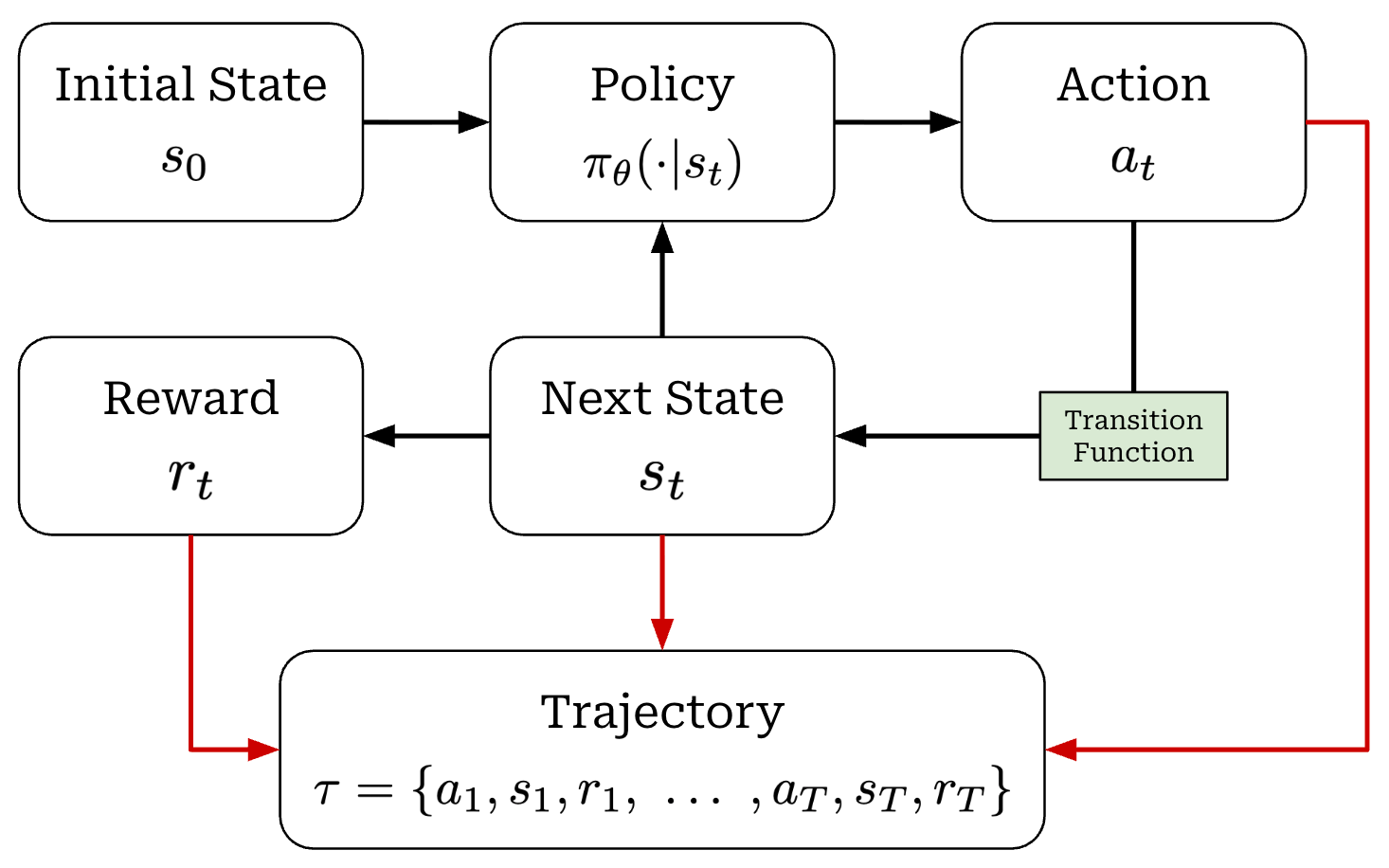
When running RL training, we have an agent that takes actions within some environment; see below.

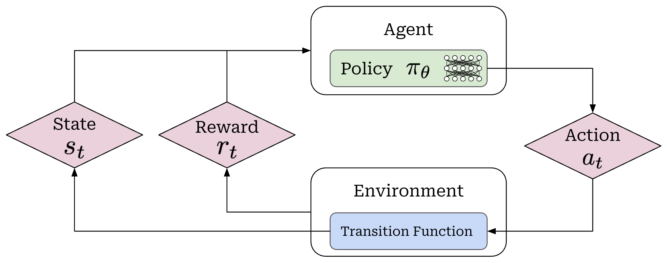
These actions are predicted by a policy—we can think of the policy as the agent’s brain—that is usually parameterized. For example, the policy is the LLM itself in the context of training LLMs. We can model the probability of a given action under our policy as π_θ(a_t | s_t). When the policy outputs an action, the state of the environment will be updated according to a transition function, which is part of the environment. We will denote our transition function as P(s_t+1 | a_t, s_t). However, transition functions are less relevant for LLMs because they are typically a pass-through; i.e., we assume s_t = {x, a_1, a_2, …, a_t}, where x is the prompt.

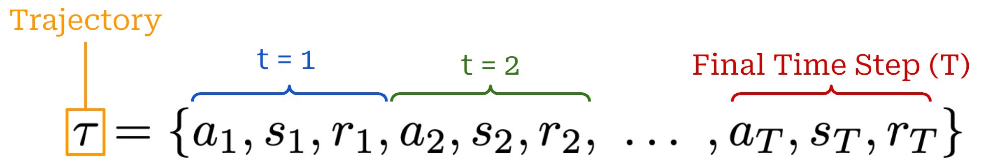
Finally, each state visited by the agent receives a reward from the environment that may be positive, negative, or zero (i.e., no reward). As shown in the prior figure, our agent acts iteratively and each action (a_t), reward (r_t), and state (s_t) are associated with a time step t. Combining these time steps together yields a trajectory; see below. Here, we assume that the agent takes a total of T steps in the environment for this particular trajectory.

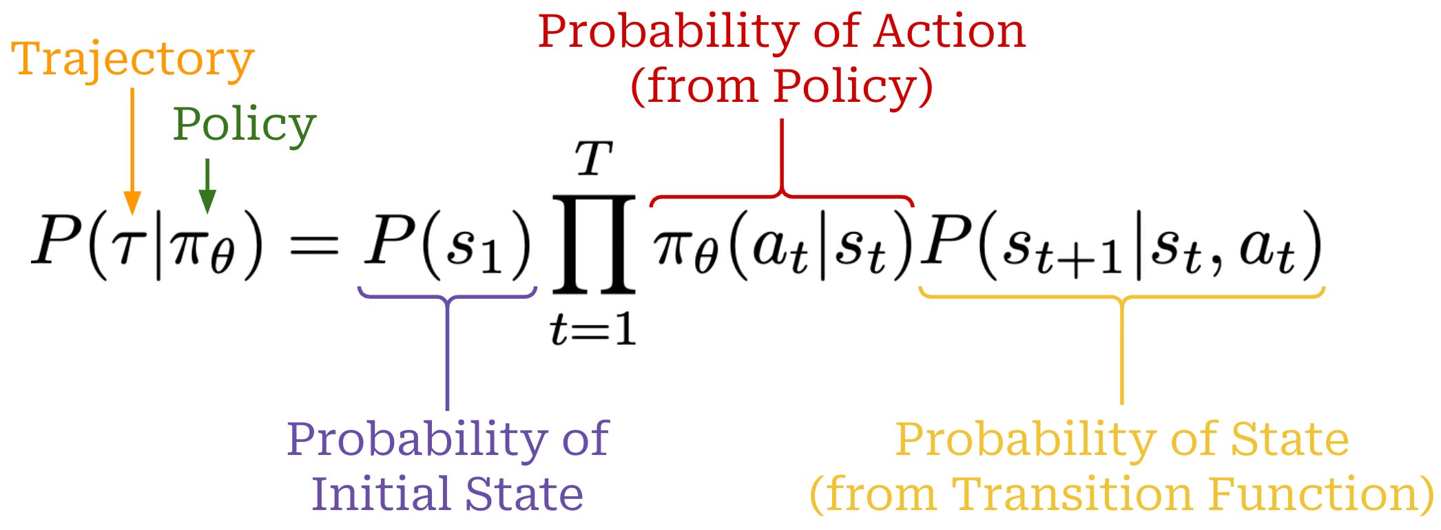
Using the chain rule of probabilities, we can also compute the probability of a full trajectory by combining the probabilities of:

Each action a_t given by our policy π_θ(a_t | s_t).
Each state s_t+1 given by the transition function P(s_t+1 | a_t, s_t).

The full expression for the probability of a trajectory is provided below.

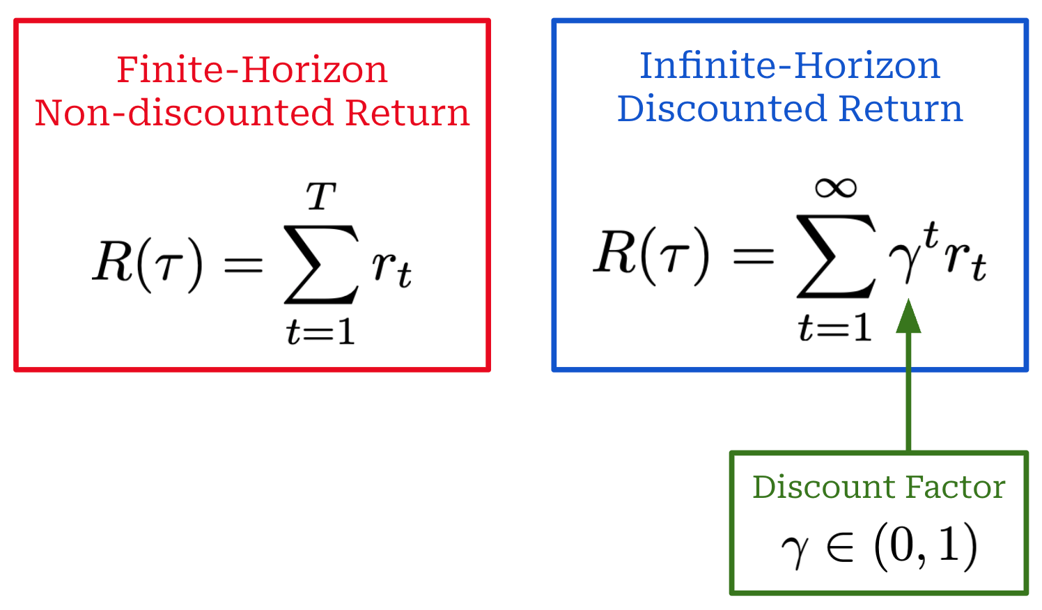
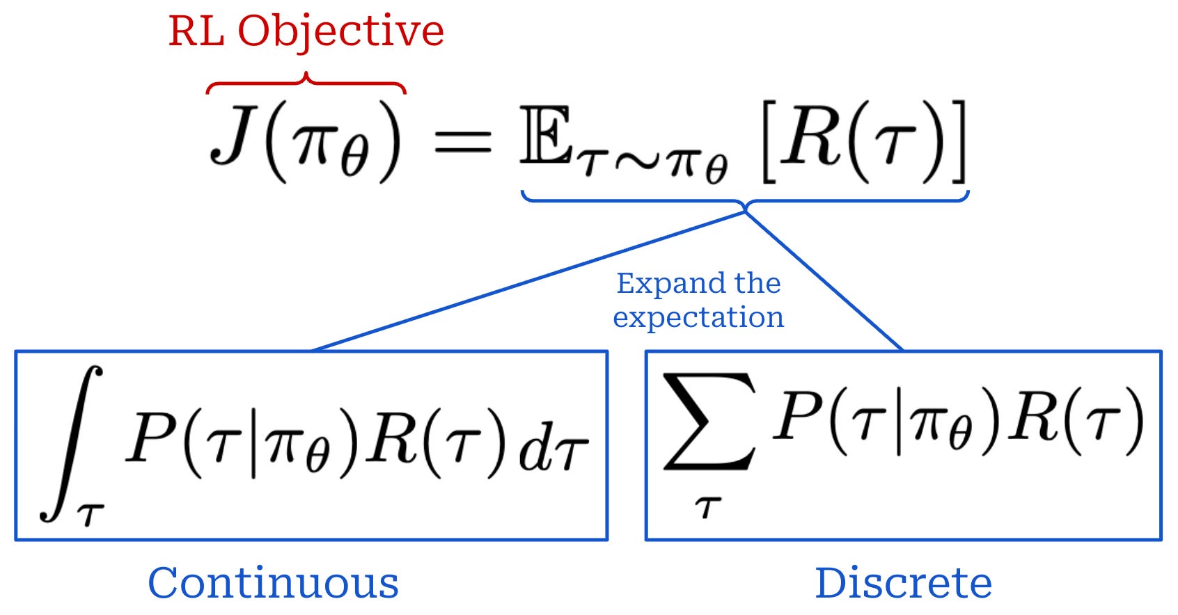
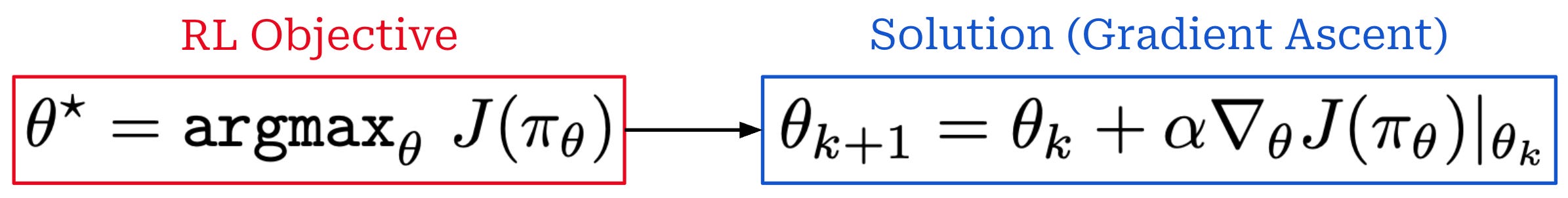
Computing the probability of a trajectory

RL objective. When training a model with RL, our goal is to maximize the cumulative reward over the entire trajectory (i.e., the sum of r_t). However, there are a few variations of this objective that commonly appear. Specifically, the reward that we maximize can either be discounted or non-discounted1; see below. By incorporating a discount factor γ, we reward our policy for achieving rewards sooner rather than later. In other words, money now is better than money later.

Our objective is usually expressed as an expected cumulative reward, where the expectation is taken over the trajectory. Expanding this expectation yields a sum over trajectories weighted by their probabilities. We can formulate this in a continuous or discrete manner; see below.

State, value, and advantage functions. Related to RL objective, we can also define the following set of functions:

Value Function V(s): the expected cumulative reward when you start in state s and act according to your current policy π_θ.
Action-Value Function Q(s, a): the expected cumulative reward when you start in state s, take action a, then act according to your policy π_θ.
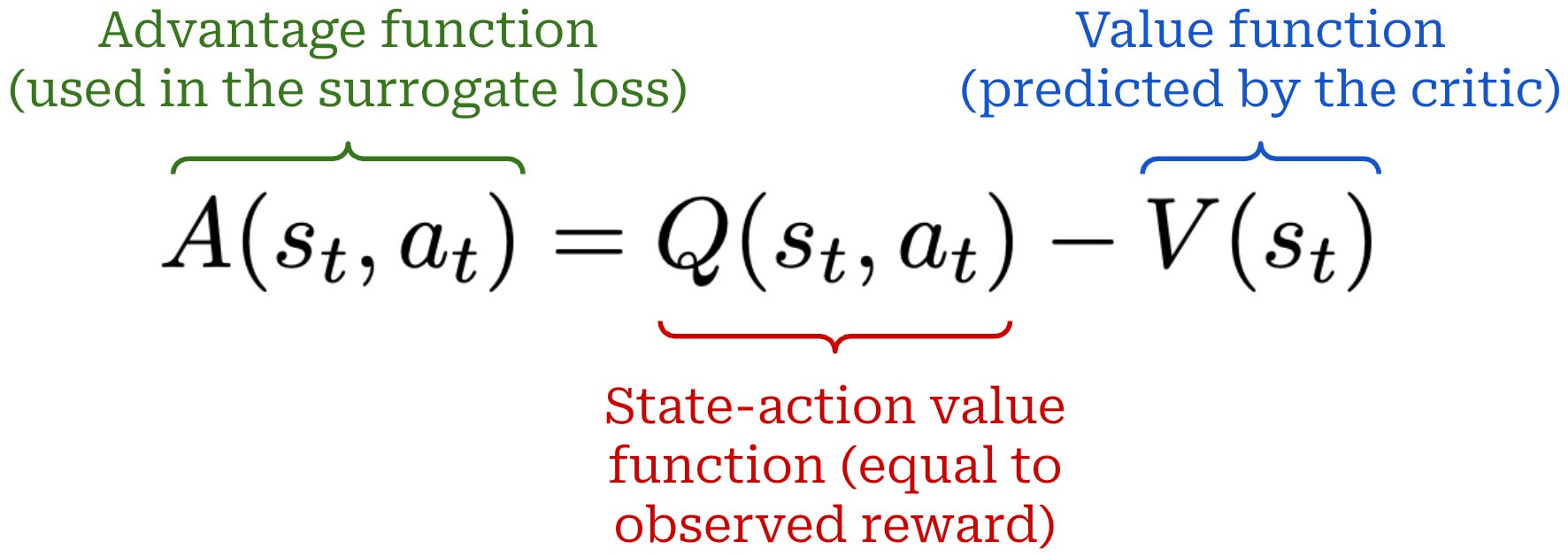
Advantage Function A(s, a): the difference between the action-value and value function; i.e., A(s, a) = Q(s, a) - V(s).

Intuitively, the advantage function tells us how useful some action a is by taking the difference between the expected reward after taking action a in state s and the general expected reward from state s. The advantage will be positive if the reward from action a is higher than expected and vice versa. Advantage functions play a huge role in RL research—they are used to compute the gradient for our policy.

“Sometimes in RL, we don’t need to describe how good an action is in an absolute sense, but only how much better it is than others on average. That is to say, we want to know the relative advantage of that action. We make this concept precise with the advantage function.” - Spinning up in Deep RL

RL Formulation for LLMs

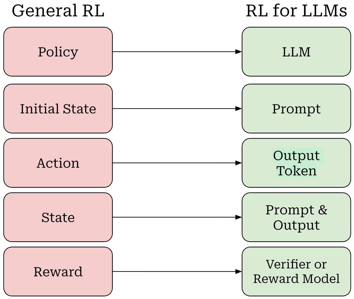
Now that we understand RL basics, we need to map the terminology that we have learned to the setting of LLM training. We can do this as follows (shown above):

Our policy is the LLM itself.
Our initial state is the prompt.
The LLM’s output—either each token or the entire completion—is an action.
Our state is the combination of our prompt with the LLM’s output.
The entire completion from the LLM forms a trajectory.
The reward comes from a verifier or reward model (more details to follow).

Notably, there is no transition function in this setup because the transition function is completely deterministic. If we start with a prompt x and our LLM predicts tokens t_1 and t_2 given this prompt as input, then our updated state simply becomes s_2 = {x, t_1, t_2}. In other words, our state is just the running completion being generated by the LLM for a given prompt x.

MDP formulation. For LLMs, there are two key ways in which RL can be formulated that differ in how they model actions:

Bandit formulation: the entire completion or response from the LLM is modeled as a single action.
Markov Decision Process (MDP) formulation: each token within the LLM’s output is modeled as an individual action.

We outlined the details for both of these formulations in a prior overview. However, PPO relies upon the MDP formulation, so we will primarily focus upon the MDP formulation here. As we should recall, an LLM generates output via next token prediction; i.e., by generating each token in the output completion sequentially. This autoregressive process is depicted below.

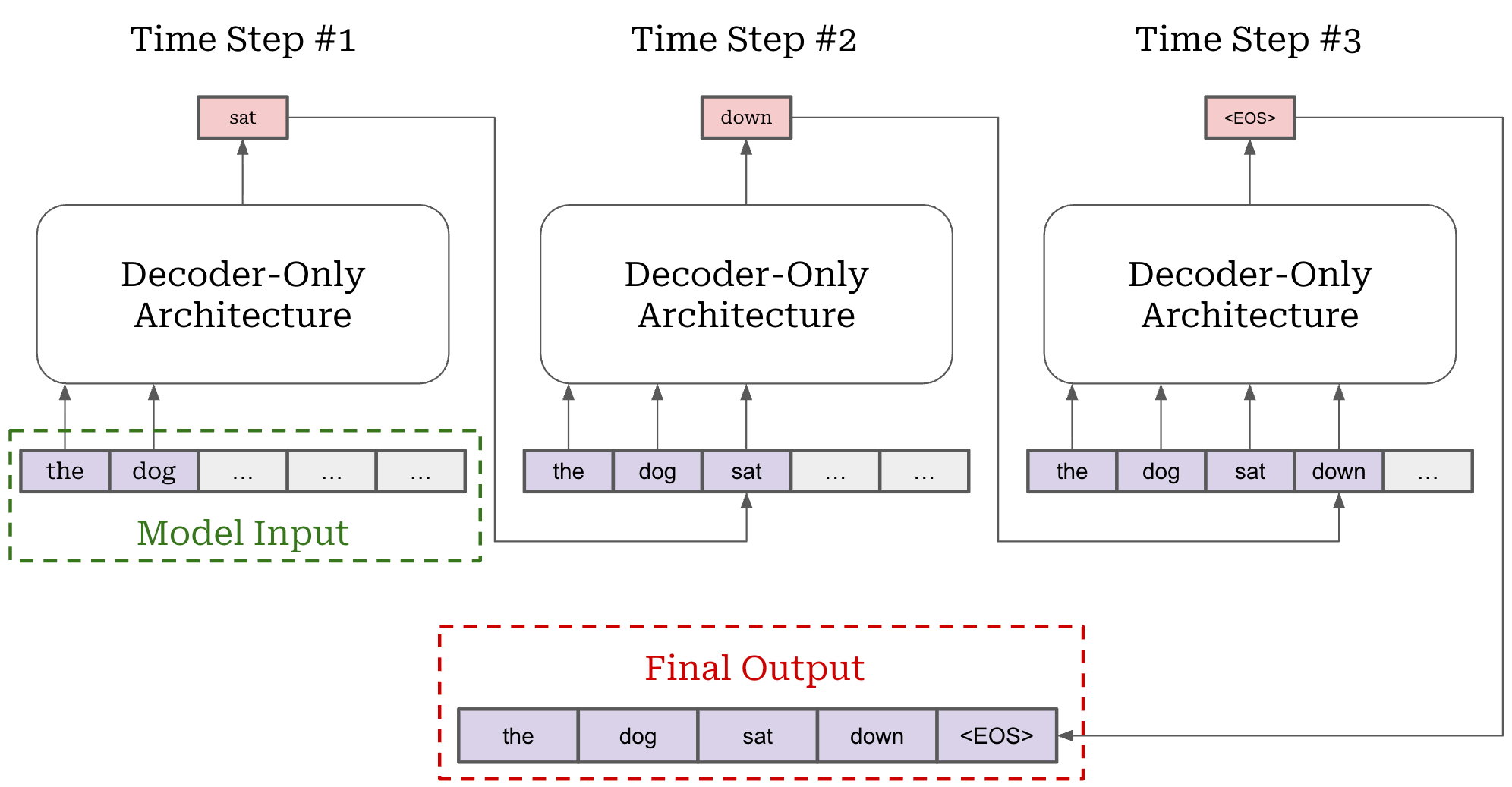
Autoregressive next token prediction with an LLM

Next token prediction maps easily to an RL setup—we can model each token as an action! This setup is called the Markov Decision Process (MDP) formulation. An MDP is a probabilistic framework for modeling decision-making that includes states, actions, transition probabilities and rewards—this is exactly the setup we have discussed so far for RL! The MDP formulation used for RL is shown below.

When modeling RL as an MDP for LLMs, our initial state is the prompt and our policy acts by predicting individual tokens. Our LLM forms a (stochastic) policy that predicts a probability distribution over tokens. During generation, actions are taken by selecting a token from this distribution—each token is its own action. After a token is predicted, it is added to the current state and used by the LLM to predict the next token—this is just autoregressive next token prediction! Eventually, the LLM predicts a stop token (e.g., <|end_of_text|> or <eos>) to complete the generation process, thus yielding a complete trajectory.

Policy Gradient Basics

During RL training, we want to maximize our objective—the cumulative (possibly discounted) reward. To accomplish this, we can just use gradient ascent; see below.

Solving the RL objective with gradient ascent

To put this in the context of LLMs, RL training follows the sequence of steps shown below. We first sample a batch of prompts and generate completions to these prompts with our LLM or policy. Then, we compute the rewards for these completions (more details to follow in later sections) and use these rewards to derive a policy update. This final policy update step is where gradient ascent is used.

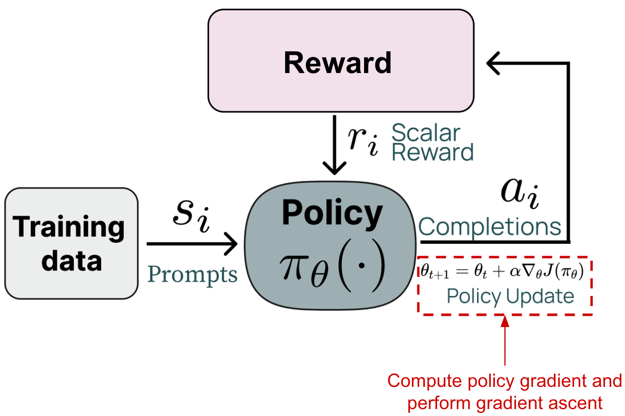
To be more specific, we use the completions and rewards to estimate the gradient of the RL training objective with respect to the parameters of our policy—this is called the “policy gradient”. If we can compute this gradient, then we can train our policy using gradient ascent. But, the question is: How do we compute this gradient?

“The goal of reinforcement learning is to find an optimal behavior strategy for the agent to obtain optimal rewards. The policy gradient methods target at modeling and optimizing the policy directly.” - Lilian Weng

Policy gradients. Nearly all RL optimizers used for LLM training (e.g., PPO [1], GRPO, and REINFORCE) are policy gradient algorithms, which operate by i) estimating the policy gradient and ii) performing gradient ascent with this estimate. These algorithms use different approaches for estimating the policy gradient, but the high-level idea behind all of them is quite similar—we just tweak small details depending on the exact technique being used. To understand policy gradient algorithms more deeply, we will first derive the simplest form of a policy gradient. Then, we will extend this idea to recover more intricate policy gradient algorithms like Trust Region Policy Optimization (TRPO) [6] and PPO [1].

The Vanilla Policy Gradient (VPG) has been extensively covered by many online resources. Other useful explanations of the VPG include:

Intro to Policy Optimization from OpenAI [link]
RLHF Book from Nathan Lambert [link]
Policy Optimization Algorithms from Lilian Weng [link]
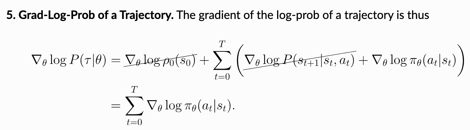
Policy Gradient Algorithms from this blog2 [link]

However, we will again derive some simple forms of the policy gradient here for completeness. As we already know, our goal in RL is to maximize cumulative rewards. If we try to compute the gradient of this objective with respect to the parameters of our policy θ, we can derive the following:

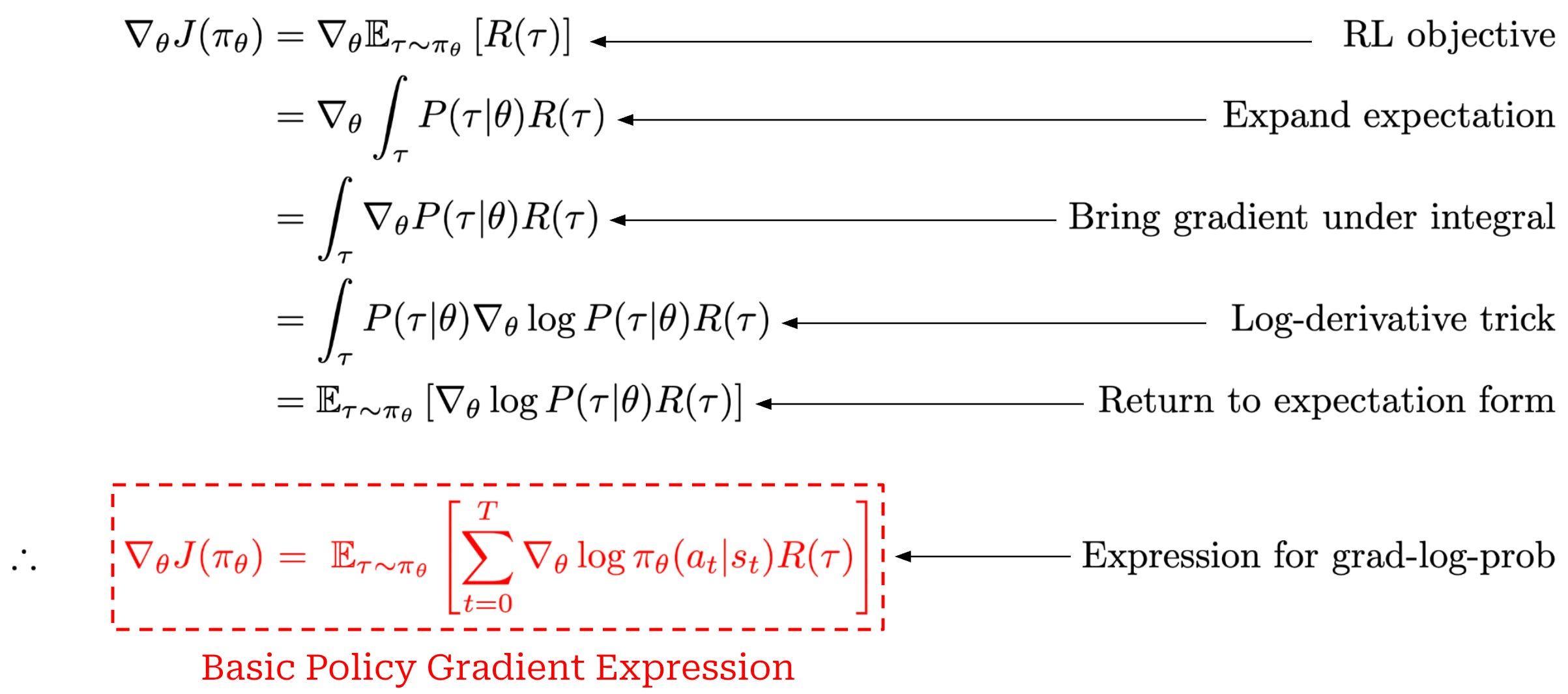
This derivation starts with the gradient of our RL training objective (cumulative reward) and ends with a basic expression for the policy gradient. The steps used in this derivation are enumerated above. The only complicated steps here are the use of the log-derivative trick and the final step, which leverages our definition for the probability of a trajectory. In the final step, we substitute in our definition for the probability of a trajectory and observe that the gradients of the initial state probability and transition function with respect to the policy parameters are always zero because neither of them depend on the policy; see below.

Implementing a basic policy gradient. The basic policy gradient expression we have derived so far is theoretical—it involves an expectation. If we want to actually compute this gradient in practice, we must approximate it with a sample mean. In other words, we sample a fixed number of trajectories—or prompts and completions in the case of an LLM—and take an average over the policy gradient expression for each of these trajectories. The basic policy gradient expression contains two key quantities that we already know how to compute:

The reward comes directly from a verifier or reward model.
Log probabilities of actions can be computed with our LLM (i.e., these are just the token probabilities from the LLM’s output).

To make the process of computing the basic policy gradient more concrete, a step-by-step implementation in PyTorch pseudocode has been provided below.

One key detail that we should notice in the above implementation is that we do not compute the policy gradient directly. Rather, we formulate a loss function for which the gradient is equal to the policy gradient then use autodiff in PyTorch to compute the policy gradient—this happens during loss.backward(). The exact loss function used to compute the policy gradient is shown below.

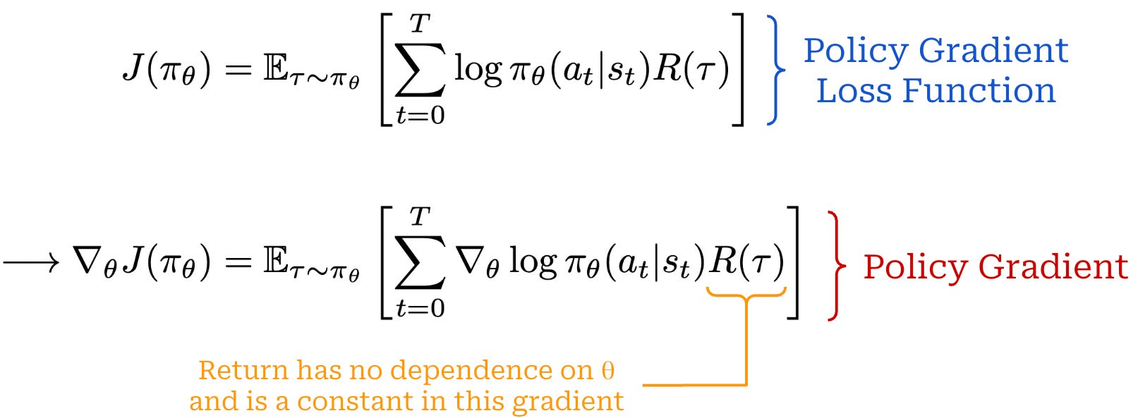
Creating a loss function for the policy gradient

This distinction is important to understand because we will formulate PPO (and TRPO!) via a loss function rather than a direct expression for the policy gradient.

Problems with the basic policy gradient. The basic policy gradient expression is straightforward, but it suffers from several notable issues:

High Variance: The gradient estimates can have high variance, making training unstable.
Unstable Policy Updates: There is no mechanism to prevent large, potentially destabilizing updates to the policy.

Due to the high variance, accurately estimating the policy gradient often requires sampling many trajectories per training iteration, which is computationally expensive. We must generate many completions with the LLM and compute the rewards and token log probabilities for all of these completions.

Additionally, this high variance increases the risk of training instability—large and inaccurate updates could potentially cause significant harm to our policy. To solve these issues, most policy gradient algorithms focus on reducing the variance of policy gradient estimates and enforcing a trust region on policy updates (i.e., limiting how much the policy can change in a single update).

“Taking a step with this gradient pushes up the log-probabilities of each action in proportion to R(𝜏), the sum of all rewards ever obtained.” - Spinning up in Deep RL

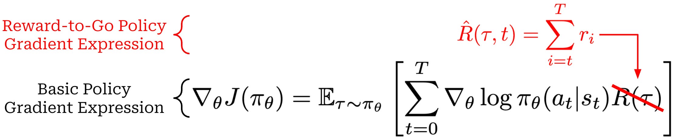
Reward-to-go. For example, we see in our basic policy gradient (copied below for reference) that we are increasing the probability of a given action based upon the cumulative reward of a trajectory. Therefore, we may increase the probability of an action due to rewards that were observed before the action even occurred!

This simple observation led to the creation of the “reward-to-go” policy gradient; see below. This modified policy gradient expression just replaces the cumulative reward with the sum of rewards observed after an action. Using the EGLP lemma, we can show that this reward-to-go formulation is an unbiased estimator of the policy gradient. Additionally, the reward-to-go policy gradient has provably lower variance compared to the basic policy gradient expression from before.

Baselines. To further reduce variance, we can also add a baseline to our policy gradient expression; see below. Similarly to the reward-to-go policy gradient, we can use the EGLP lemma to show that a baselined version of our policy gradient is unbiased and has lower variance. Due to the EGLP lemma, this baseline must only depend upon the current state (i.e., otherwise an assumption of the EGLP lemma is violated and the proofs are no longer valid).

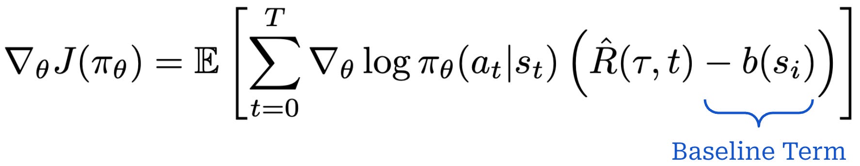
Adding a baseline to our policy gradient expression

This expression is nearly identical to the reward-to-go policy gradient—we just subtract an additional baseline from the reward-to-go term. There are many possible choices for baselines that can be used in policy gradient estimates. One common baseline is the value function. Using the value function as a baseline positively reinforces actions that achieve a cumulative reward that is higher than expected.

A common problem with vanilla policy gradient algorithms is the high variance in gradient updates… In order to alleviate this, various techniques are used to normalize the value estimation, called baselines. Baselines accomplish this in multiple ways, effectively normalizing by the value of the state relative to the downstream action (e.g. in the case of Advantage, which is the difference between the Q value and the value). The simplest baselines are averages over the batch of rewards or a moving average. - RLHF book

Generic policy gradient. In [3], the options for computing the policy gradient were summarized with a more generic policy gradient expression; see below.

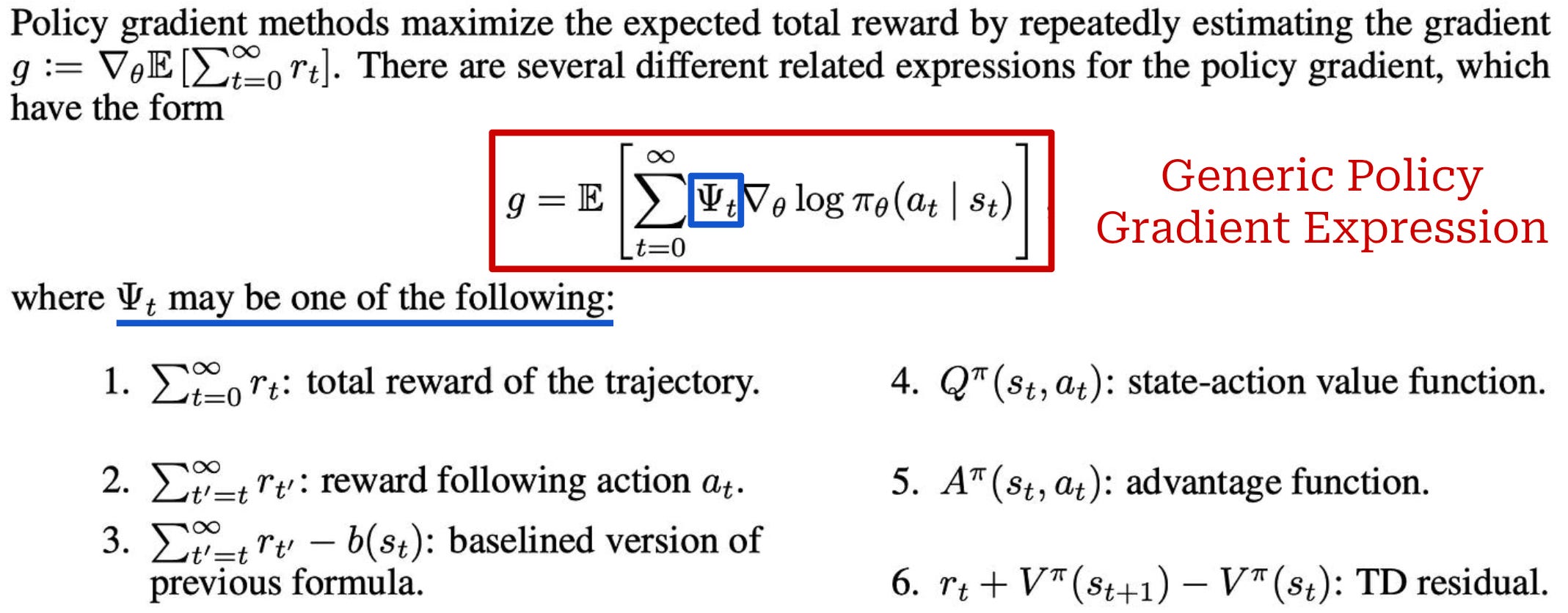
This expression is nearly identical to expressions we have seen so far. The only difference is that we have changed our reward term R(𝜏) to a generic Ψ_t term, which can be set equal to several different expressions. For example, we can:

Set Ψ_t = R(𝜏) to recover our basic policy gradient expression.
Set Ψ_t equal to rewards received after time t to recover our reward-to-go variant of the policy gradient.
Set Ψ_t equal to a baselined version of the reward; e.g., the difference between cumulative reward R(𝜏) and the value function V(s_t).
Set Ψ_t equal to the state-action (Q) or advantage function (A).

Despite the many possible formulations, PPO—and nearly all of the RL optimizers used in the domain of LLMs—focuses upon setting Ψ_t equal to the advantage function A(s_t, a_t). This setting is referred to as the vanilla policy gradient (VPG); see below. In theory, the VPG yields the lowest-variance gradient estimate.

Although the VPG has low variance, there is still no mechanism to enforce a trust region in the policy update—a large and destructive policy update can still destabilize the training process. PPO was created as a solution to this problem. As we will see, PPO resembles the basic policy gradient expressions we have seen but has added mechanisms for enforcing a trust region on the policy update. We will now learn more about PPO and the many practical details involved in its implementation.

Proximal Policy Optimization (PPO)

Now that we understand RL basics, we will spend the next section learning about Proximal Policy Optimization (PPO) [1]. This explanation will build upon the VPG expression that we derived in the last section, beginning with Trust Region Policy Optimization (TRPO) [6]—a predecessor to PPO. TRPO is effective at stabilizing training, but it is also relatively complex. PPO was developed as a more practical alternative with similar benefits. To conclude the section, we will also cover Generalized Advantage Estimation (GAE) [3], which is the most common approach for computing the advantage function in PPO.

Trust Region Policy Optimization (TRPO) [6]

“TRPO uses a hard constraint rather than a penalty because it is hard to choose a single value of β that performs well across different problems—or even within a single problem, where the characteristics change over the course of learning.” - from [1]

Prior to learning about PPO, we need to take a look at its predecessor, Trust Region Policy Optimization (TRPO) [6]. The key motivation behind TRPO is creating an algorithm that is data efficient and does not require too much hyperparameter tuning. To do this, authors in [6] propose the constrained objective below, which is guaranteed to monotonically improve our policy. This objective enforces a trust region on the policy update, thus eliminating the risk of large and destructive policy updates that could destabilize training.

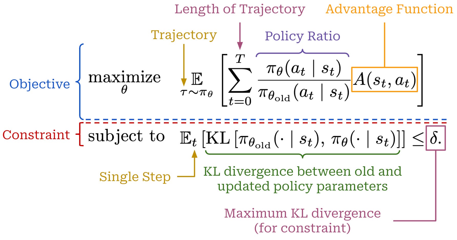
Surrogate objective. This objective shown above is called the surrogate objective in TRPO. This naming stems from the fact that the surrogate objective is different from the standard RL training objective. In RL, we aim to maximize cumulative reward, but—as we have seen in our discussion of the VPG—directly maximizing this “true” objective of RL can lead to training instability. TRPO formulates the surrogate objective to maximize in place of the true objective.

There are a few noticeable differences between the above expression for TRPO and the VPG:

Action probabilities in the current policy are normalized by the probability of that action in the old policy (i.e., the policy prior to training)—this forms the policy ratio (also called an importance ratio). We also use probabilities in this formulation instead of log probabilities.
There is a constraint placed on the objective to ensure that the expected KL divergence between the new and old policies is less than a threshold δ.

Otherwise, the TRPO loss function shares a similar structure to that of VPG—it includes the advantage function and a sum over token-level probabilities in a trajectory.

Policy ratio. The centerpiece of the TRPO loss function is the policy ratio, defined as shown below. The policy ratio tells us how much more likely a given action is in our current policy relative to the probability of that action before the training process started—this is denoted as the “old” policy.

This quantity serves the purpose of assigning an importance to different actions within our trajectory. If the new policy assigns a higher probability to an action than the old policy did, this ratio is greater than one, increasing the influence of that action’s advantage in the objective. Conversely, if the new policy assigns a lower probability, the ratio is less than one, reducing the influence of that action. The policy ratio ensures that the policy update emphasizes actions that the new policy is making more likely—especially if those actions have high advantage—while suppressing actions that are becoming less likely under the new policy. By doing this, we ensure that the update is properly weighted according to how the new policy differs from the old, enabling stable and efficient policy improvement.

Solving the surrogate objective. Although this objective yields stable policy updates, solving it can be quite involved. By introducing an explicit constraint into our objective, we eliminate the ability to solve this objective with simple gradient ascent3. Instead, we have to solve this objective via the more complex conjugate gradient algorithm. Alternatively, we could remove this constraint and instead add the KL divergence as a penalty into our loss function; see below. This unconstrained loss is simpler and can again be solved with basic gradient ascent.

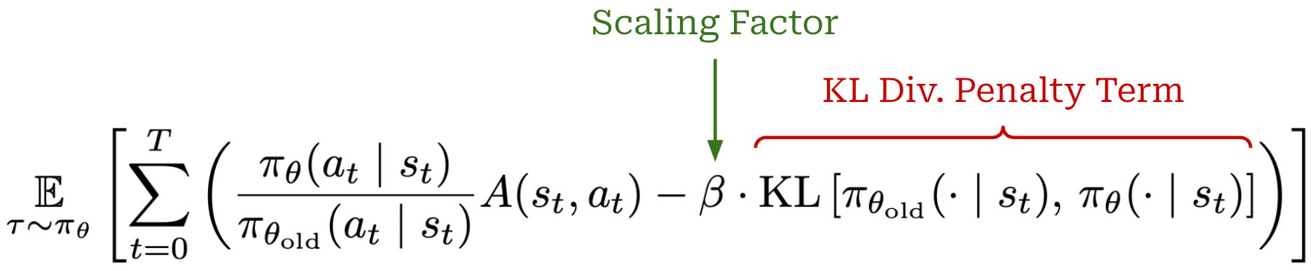
From TRPO to PPO. Formulating the constraint from TRPO as a penalty allows us to avoid complicated optimization techniques and rely upon basic gradient ascent. However, a new hyperparameter β is introduced to the optimization process that makes tuning difficult. Properly setting the value of β is essential for this objective to perform well, and finding a single value of β that generalizes to many domains is hard. As a result, both of the above objectives have their issues:

The TRPO surrogate objective is too complex to solve in practice.
The reformulated penalty objective is sensitive to the setting of β.

We want to develop an algorithm that retains the benefits of TRPO—such as stability, data efficiency, and reliability—while avoiding its complexity. Ideally, the algorithm should be broadly applicable and solvable using basic gradient ascent. These goals led to the proposal of PPO, which is largely inspired by TRPO. PPO’s objective is inspired by the TRPO surrogate objective but replaces the hard KL constraint with a clipping mechanism to enforce a trust region in a simpler way.

Proximal Policy Optimization Algorithms [1]

“We propose a new family of policy gradient methods for RL, which alternate between sampling data through interaction with the environment, and optimizing a surrogate objective function using stochastic gradient ascent.” - from [1]

The VPG is simple to compute in practice, but it has poor data efficiency (i.e., the model must be trained over many samples to perform well) and high variance in the policy updates. These problems are largely solved by TRPO but at the cost of significant added complexity. PPO is an algorithm with the data efficiency and reliability benefits of TRPO that is still solvable with gradient ascent. In this way, PPO is a simpler algorithm compared to TRPO. As we will see, however, PPO is still a complex algorithm with many implementation complexities of its own.

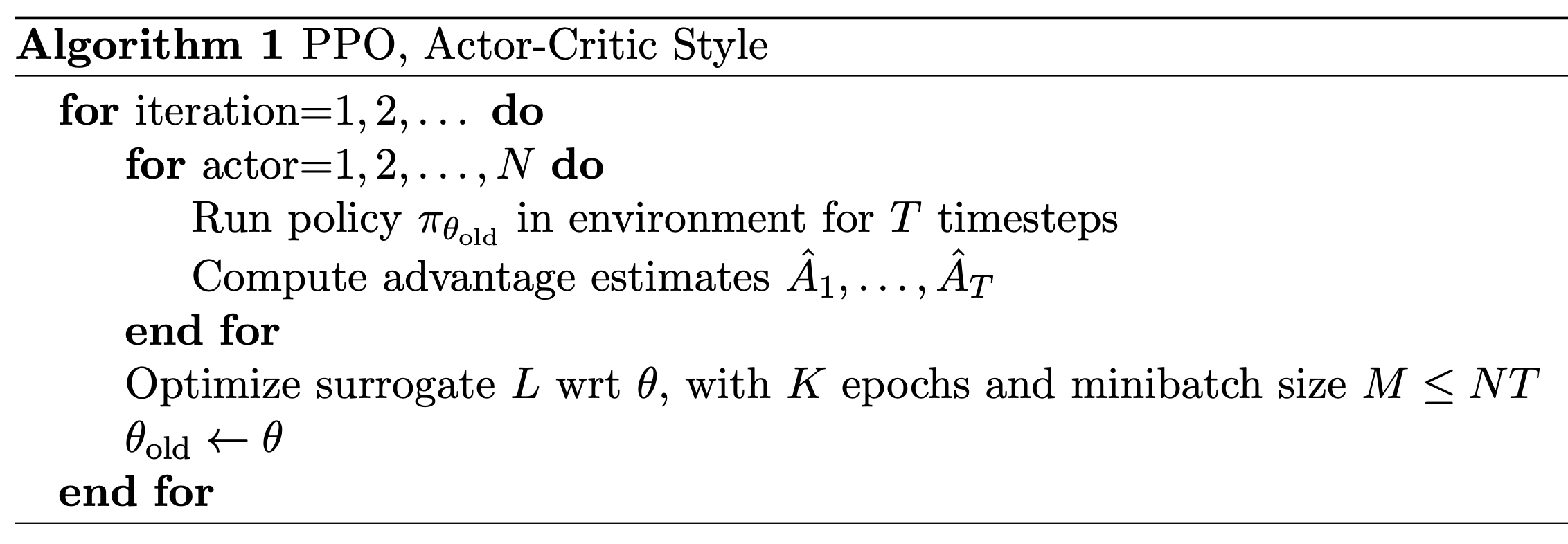
Training process. Similarly to TRPO, PPO focuses upon optimizing a surrogate objective, but the objective in PPO has no constraint and has been slightly modified. As shown in the algorithm above, PPO performs more than a single policy update in each step, instead alternating between:

Sampling new data or trajectories from the policy.
Performing several epochs of optimization on the sampled data.

The PPO surrogate objective is again based upon the policy ratio between the current policy and the old model (i.e., the policy before any training is performed). To match notation in [1], we will denote the policy ratio as r_t(θ), which is similar to the r_t notation used for the reward for time step t. However, the policy ratio is unrelated to the reward! To obtain the PPO objective, we start with the surrogate objective being maximized by TRPO with no KL constraint; see below.

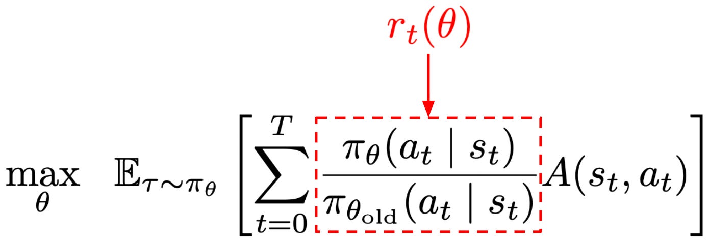
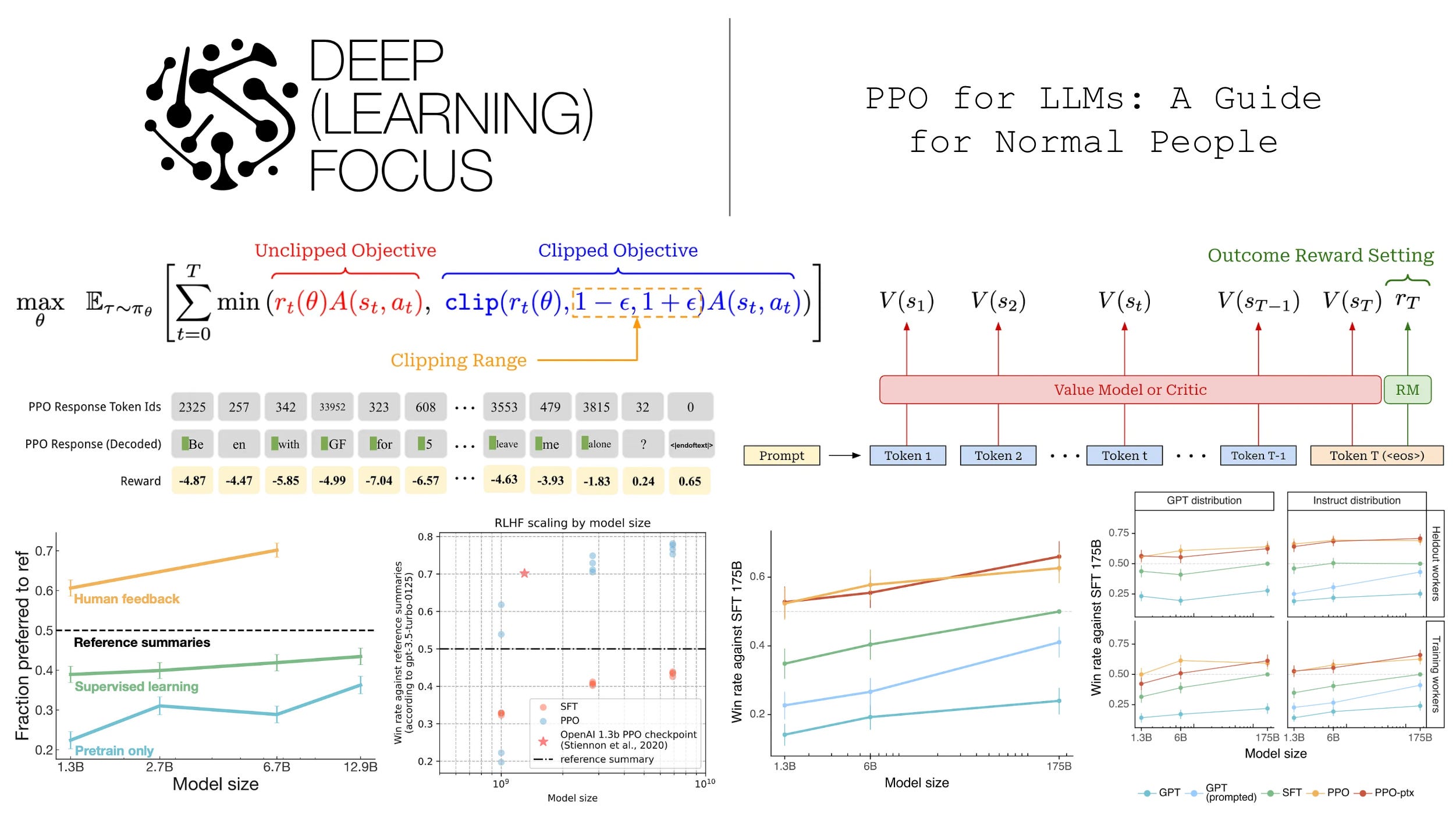
We will call this formulation the “unclipped” objective. Because it does not have a constraint, this objective can be easily computed to derive the policy gradient by i) estimating the advantage and ii) computing the policy ratio. However, if we try to maximize this unconstrained objective, this will potentially lead to large and destructive policy gradient updates that make the training process unstable. To solve this issue, PPO introduces a novel clipping mechanism into the surrogate objective that helps us with maintaining the trust region; see below.

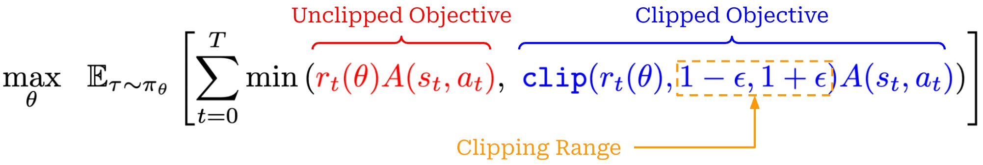
The main term in the objective is unchanged, but there is an added term with a clipped version of the policy ratio—the policy ratio must fall in the range [1 - ε, 1 + ε]4. The clipping term disincentivizes the RL training process from moving the policy ratio away from a value of one. The PPO surrogate objective takes the minimum of clipped and unclipped objectives. In this way, the PPO objective is a pessimistic (lower) bound for the original, unclipped objective5.

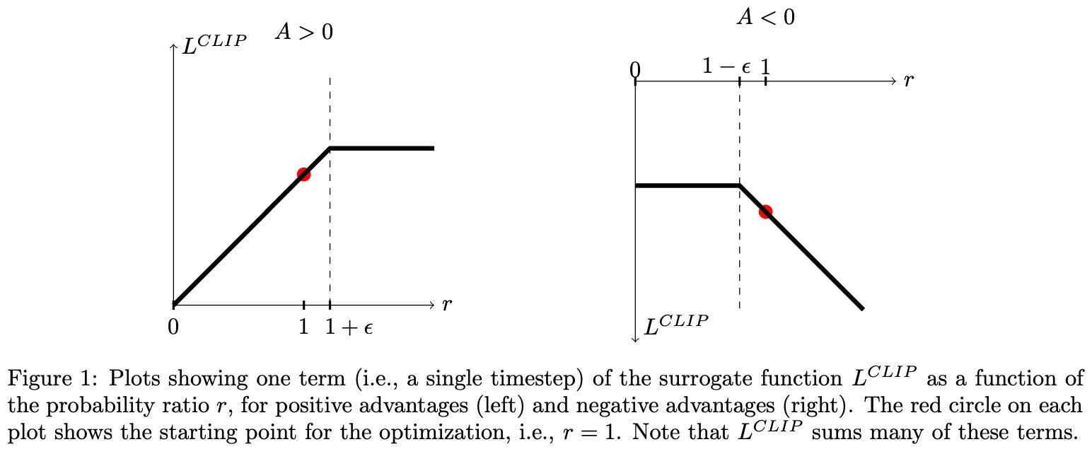
Depending upon whether the advantage is positive or negative, the behavior of clipping is slightly different; see above. The use of a minimum in the surrogate objective causes clipping to be applied in only one direction. In particular, we can arbitrarily decrease surrogate objective by moving the policy ratio far away from a value of one, but clipping prevents arbitrarily increasing the objective via the policy ratio. In this way, PPO de-incentivize large policy ratios so that our policy does not deviate too much from the old policy after training updates.

“With this scheme, we only ignore the change in probability ratio when it would make the objective improve, and we include it when it makes the objective worse.” - from [1]

To more deeply understand the clipping logic of PPO, we can consider each of the four possible cases that can arise when optimizing the surrogate objective:

Case #1 [A > 0, r_t(θ) ≤ 1 + ε]: advantage is positive—this is an action that we want to reinforce. Our policy ratio is below 1 + ε, so we perform a normal policy gradient update to increase the probability of this action.
Case #2 [A > 0, r_t(θ) > 1 + ε]: advantage is positive again, but our policy ratio is greater than 1 + ε. This means that this action is already more likely in the new policy relative to the old policy. The objective gets clipped, and the gradient with respect to further increases in the policy ratio is zero. This prevents the policy from making the action even more likely
Case #3 [A < 0, r_t(θ) ≥ 1 - ε]: advantage is negative—this is an action we want to negatively reinforce (i.e., decrease probability). Our policy ratio is above 1 - ε, so we perform a normal policy gradient update to decrease the probability of this action.
Case #4 [A < 0, r_t(θ) < 1 - ε]: advantage is negative again, but our policy ratio is less than 1 - ε. This means that this action is already less likely in the new policy relative to the old policy. The objective gets clipped, and the gradient with respect to further decreases in the policy ratio is zero. This prevents the policy from making the action even less likely.

The policy ratio is computed between the current and old policies. The old policy is updated to match the current policy each time new data is sampled in PPO. In the context of LLMs, we perform 2-4 gradient updates (or sometimes more) [2] for each batch of data, so the old model is updated frequently. The clipping operation in PPO, therefore, maintains a trust region for a particular batch of data.

KL divergence. When training LLMs with PPO, we usually incorporate the KL divergence between the current policy and a reference policy—usually some policy from before RL training begins (e.g., the SFT model)—into the training process. This added KL divergence term penalizes the policy from becoming too different from the reference policy, which has a regularizing effect. We compute KL divergence per token by comparing the token probability distributions outputted by the two LLMs for each token within the sequence. Details on how exactly the KL divergence is computed in practice can be found here.

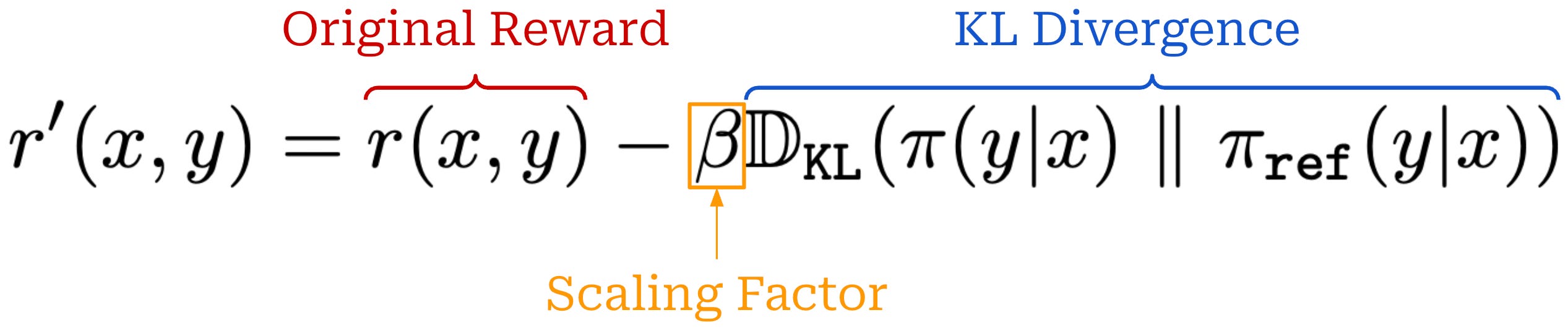
Incorporating KL divergence into the reward

There are two common ways of adding the KL divergence into PPO training. First, we can directly subtract the KL divergence from the reward in RL; see above. Alternatively, we can add the KL divergence as a penalty term to the RL training objective as shown below. In both cases, we simply want to maximize rewards without making our new policy too different from the reference.

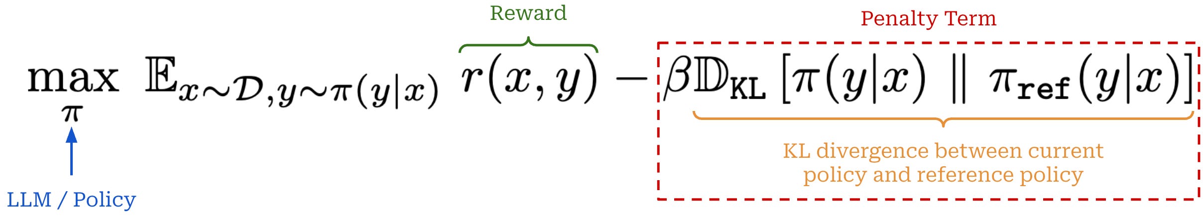
Incorporating a KL penalty into the RL training objective

Such a KL divergence term is almost universally used in RL training for LLMs, though the exact implementation varies. Both of the approaches outlined above have been used successfully. However, capturing the KL divergence via a penalty term in the training objective is probably more common (and a bit simpler).

The critic. Recall that the advantage function is defined as the difference between the state-action value function and the value function. In PPO, we estimate the state-action value function—the expected reward for taking a specific action in a given state—by using the actual reward observed for a trajectory. The value function, in contrast, is typically estimated using a learned model; see below.

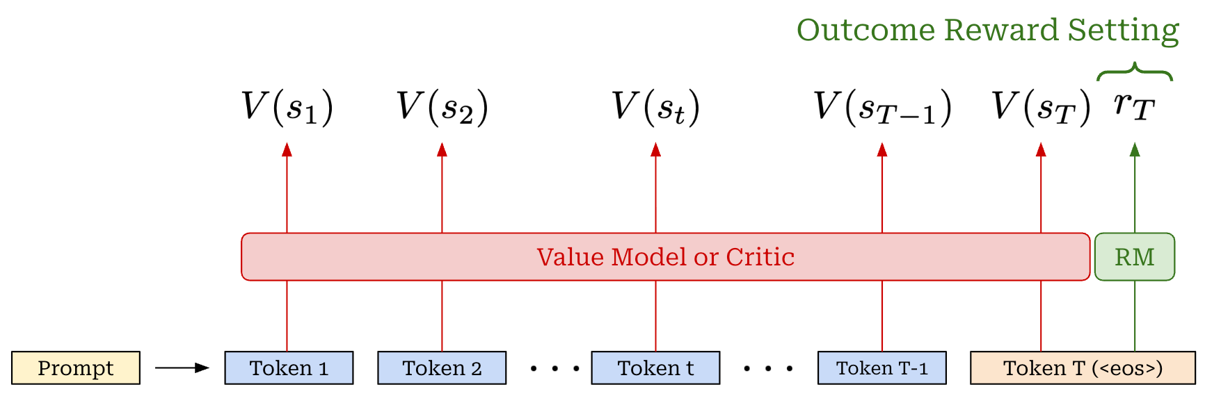
For example, we can create a separate copy of our policy, or—for better parameter efficiency—add a dedicated value head that shares weights with the policy to predict the value function. This learned value function is often referred to as a value model or critic. Taking a partial response as input, the critic predicts the expected final reward for every token position within the sequence; see below.

Critic versus reward model. In the context of LLMs, we predict the reward with a reward model. Additionally, most LLMs are trained using outcome supervision, meaning that a reward is only assigned after the model has generated a complete response (i.e., after the <eos> token has been outputted). The critic and reward model are similar in that they are both learned models—usually another copy of our LLM policy—that predict rewards. However, the critic predicts expected rewards given a partial completion as input, while the reward model typically predicts the reward received by an entire response; see below. Going further, the reward model is fixed throughout RL training, while the critic is continually updated.

Critic training. The value function is on-policy—it is dependent upon the current parameters of our policy. Unlike reward models which are fixed at the beginning of RL training, the critic is trained alongside the LLM in each policy update to ensure that its predictions remain on-policy—this is called an actor-critic setup6. This is accomplished by adding an extra mean-squared error (MSE) loss—between the rewards predicted by the critic and actual rewards—to the surrogate loss.

PPO implementation. To make each of these ideas more complete, we have implemented PPO in PyTorch pseudocode below. In this implementation, we see several of the key ideas we have discussed so far, such as:

Computing the KL divergence between the current policy and a reference model, then directly subtracting this KL divergence from our reward.
Using a learned critic to compute the advantage (and training this critic via an MSE loss alongside the policy itself).
Computing the policy ratio with respect to the old model. The script below performs a single policy update, but PPO usually performs several (i.e., 2-4 in the case of LLMs [2]) policy updates for each batch of data. The “old” model in the policy ratio is the model from before the first update for a batch.
Computing the full (clipped) PPO loss. We take the negative of this loss because PyTorch performs gradient descent (not ascent) by default.
Aggregating or averaging the token-level PPO loss across a batch of sequences. There are many ways to aggregate the loss in a batch, and the approach used can significantly impact results [2]7.

One interesting detail we see here is that—despite the PPO loss using token probabilities and not log probabilities—we choose to work with token log probabilities and exponentiate them instead of using raw probabilities when computing the policy ratio. This is a commonly-used numerical stability trick.

import torch
import torch.nn.functional as F

# constants
kl_beta = 0.1
critic_weight = 0.5
ppo_eps = 0.2

# sample prompt completions and rewards
with torch.no_grad():
    completions = LLM.generate(prompts)  # (B*G, L)
    rewards = RM(completions)  # (B*G, 1)

# create a padding mask from lengths of completions in batch
completion_mask = <... mask out padding tokens ...>

# compute value function / critic output
values = CRITIC(completions)  # (B*G, L) - predicted reward per token!

# get policy logprobs for each action
llm_out = LLM(completions)
per_token_logps = F.log_softmax(llm_out, dim=-1)  # (B*G, L)

# get reference logprobs for each action
ref_out = REF(completions)
ref_per_token_logps = F.log_softmax(ref_out, dim=-1)  # (B*G, L)

# compute KL divergence between policy and reference policy
kl_div = per_token_logps - ref_per_token_logps

# directly subtract KL divergence from rewards
# NOTE: KL div is per token, so reward becomes per token and reward
# for all tokens (besides last token) is just kl divergence.
# Reward for last token is sum of outcome reward and KL div.
rewards -= kl_beta * kl_div # (B*G, L)

# compute the advantage - simple approach
advantage = rewards - values.detach()  # (B*G, L)

# compute the policy ratio
# NOTE: old_per_token_logps must be persisted during first policy
# update for this batch of data and re-used in each subsequent update
policy_ratio = torch.exp(
    per_token_logps - old_per_token_logps,
)  # (B*G, L)
clip_policy_ratio = torch.clamp(
    policy_ratio,
    min=1.0 - ppo_eps,
    max=1.0 + ppo_eps,
)

# compute the ppo loss
ppo_loss = torch.min(
    advantage * policy_ratio,
    advantage * clip_policy_ratio,
)  # (B*G, L)
ppo_loss = -ppo_loss

# combine ppo loss and critic mse loss
critic_loss = ((rewards - values) ** 2)  # (B*G, L)
loss = ppo_loss + critic_weight * critic_loss

# aggregate the loss across tokens (many options exist here)
loss = ((loss * completion_mask).sum(axis=-1) /
        completion_mask.sum(axis=-1)).mean()

# perform policy gradient update
optimizer.zero_grad()
loss.backward()
optimizer.step()

Experiments. The LLM setting is not considered in [1], as PPO was proposed during the heyday of DeepRL—well before the proliferation of LLMs. Understanding the experimental results in [1] is nonetheless useful for gaining intuition on the mechanics of PPO. In these experiments, PPO is used to train fully-connected multi-layer perceptrons (MLPs) from scratch on a variety of robotics and video game tasks. The policy and critic are kept separate (i.e., no parameter sharing).

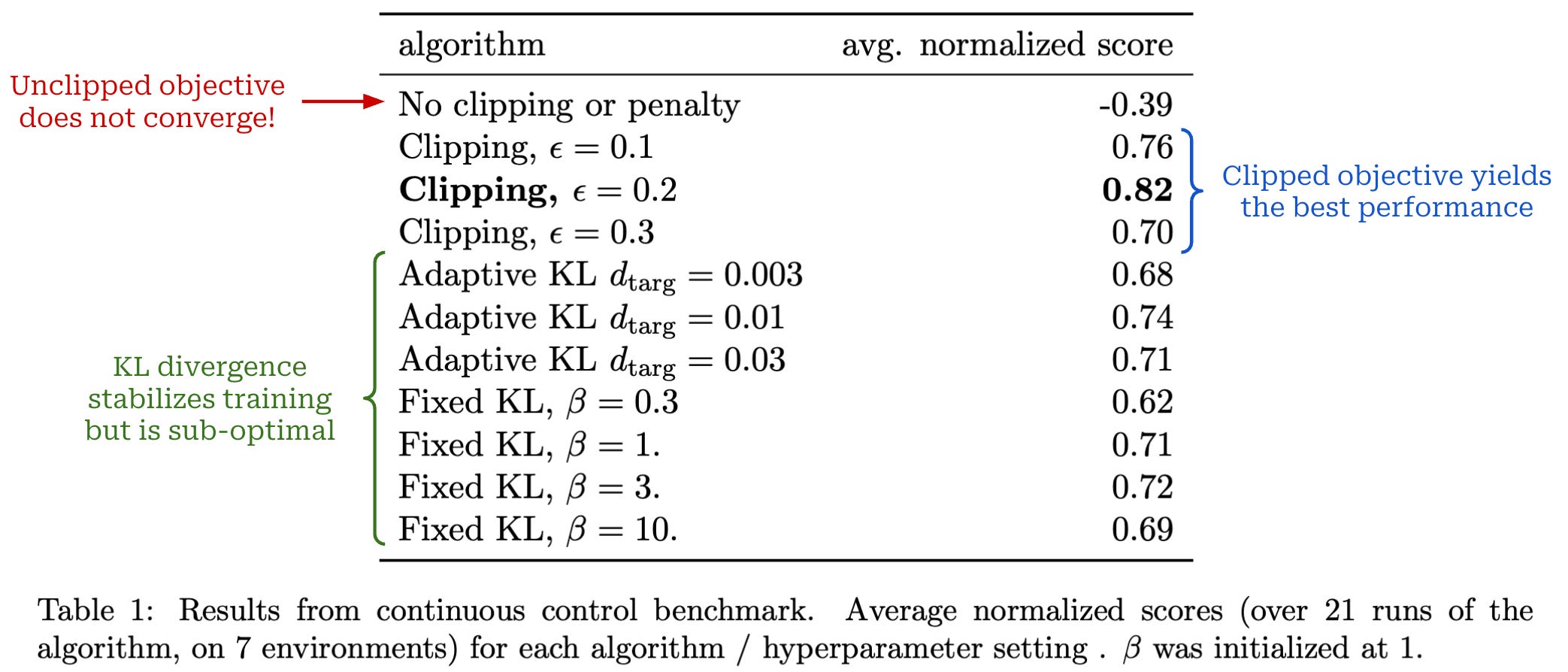
First, authors use several simulated robotics tasks from the OpenAI Gym to test different formulations of the surrogate loss in PPO:

The clipped objective (standard for PPO).
The unclipped objective.
The unclipped objective with (adaptive8) KL divergence.

Unlike the typical RL training setup for LLMs, these experiments compute the KL divergence between the current policy and the old model, with the goal of testing whether this approach works better than the standard PPO clipping mechanism. Ordinarily, when training LLMs with PPO, the KL divergence is computed between the current policy and a reference model (e.g., the SFT model), not the old model9. However, in these experiments, using a reference model for the KL divergence is not possible because we are training models from scratch—there is no pretrained model to serve as a reference.

The results from testing these different objectives are outlined below—the clipped objective for PPO stabilizes training and clearly outperforms the other options.

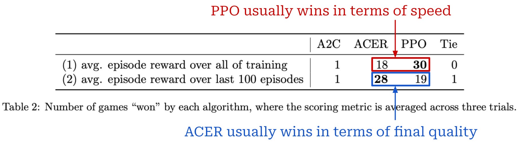
PPO is also tested on 49 games in the Atari gameplay domain and compared to strong baseline RL algorithms like A2C and ACER. Performance is measured based on two metrics:

Average reward throughout training (favors faster learning).
Average reward over the last 100 training steps (favors final quality / reward).

For each of these metrics, we compute a “win rate”, which captures the number of times each algorithm achieves the top score across all Atari games. The results of these experiments are shown below, where we see that baseline algorithms like ACER perform similarly to or better than PPO but learn much slower. PPO stabilizes training, performs well, and yields an improvement in sample complexity10.

Generalized Advantage Estimation (GAE) [3]

The advantage tells us how much better a given action is compared to the average action in a given state: A(s_t, a_t) = Q(s_t, a_t) - V(s_t). The value function in this formulation is estimated by our critic, but we have not yet discussed in detail how the advantage function can be computed. In PPO, the advantage function is estimated on a per-token (or action) basis. There are two main approaches that can be used to compute the advantage, and these approaches form the basis for most other techniques.

(1) Monte Carlo (MC). An MC estimate of the advantage relies upon the actual reward observed for the full trajectory. Namely, the advantage is computed as the difference between the cumulative reward for the full trajectory R(s_t)11 and the value function for the current state V(s_t), as predicted by the critic.

So far, our discussions of PPO have assumed an MC approach for estimating the advantage. The MC estimate has low bias because it relies on the actual reward observed for the trajectory (exact information), but MC estimates also have high variance. Therefore, we need to take many samples and make a sufficient number of observations to yield an accurate advantage estimate—this can be expensive.

(2) Temporal Difference (TD). The TD residual uses per-token value predictions from the critic to form a one-step estimate of the advantage, as shown below.

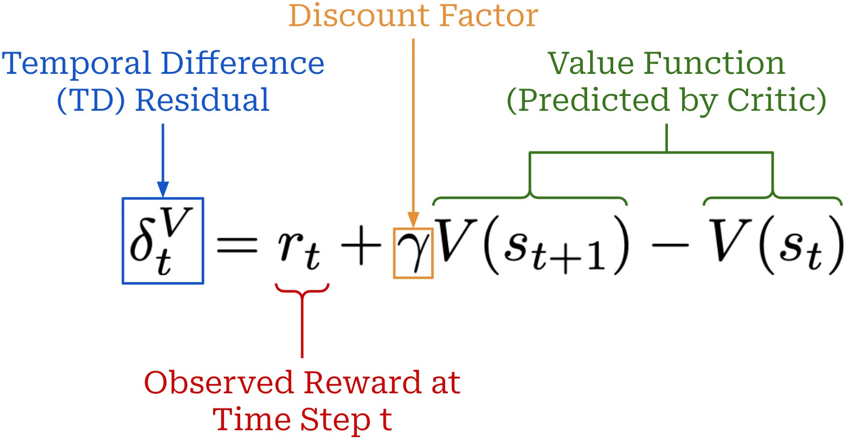
This TD residual analyzes how much the expected reward changes after predicting a single token and observing the actual reward for that action12. We subtract the value for the current state V(s_t) from the sum of:

The observed reward for the current state r_t.
The (discounted) value of the next state V(s_{t+1}).

Similarly to V(s_t), the sum of these two terms captures the expected return at state s_t. However, the reward for the current state is captured via the actual observed reward r_t rather than being estimated by the critic. Therefore, the difference between these terms is capturing how much better the actual reward observed at state s_t is than expected—this is the advantage!

By using the actual reward r_t, we incorporate some exact information into our advantage estimate—the terms in the estimate come partly from our critic and partly from real rewards. Using such token-level rewards to estimate the advantage lowers the variance of the policy gradient. If our value function were exact, then the TD residual would also form an unbiased advantage estimate. Unfortunately, we do not have access to the ground truth value function, so we train a critic to estimate the value function13. Because accurately anticipating final rewards from a partial response is difficult, the TD residual is biased.

N-step estimators. The TD residual analyzes the difference between actual and expected reward for a single step. However, we can generalize this idea to capture any number of steps. As shown below, an N-step advantage estimator has a similar structure to the TD residual, but it incorporates real rewards for N states, where N can be greater than one.

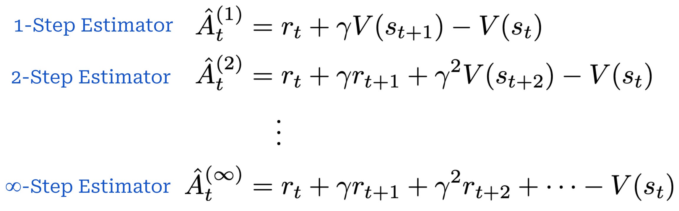
Similarly to the single-step TD residual, advantage estimators with lower values of N have low variance but high bias. As we increase the value of N, however, we are incorporating more exact reward information into the advantage estimate, thus lowering the bias (and, in turn, increasing variance).

Taking this further, we can even recover an MC estimate by setting N equal to the total number of steps in the trajectory! This setting of N simply yields the difference between cumulative reward and the value of the current state V(s_t). Therefore, different settings of N yield different tradeoffs in bias and variance, spanning all the way from the single-step TD residual (high bias, low variance) to an MC estimate (high variance, low bias).

“GAE is an alternate method to compute the advantage for policy gradient algorithms that better balances the bias-variance tradeoff. Traditional single-step advantage estimates can introduce too much bias, while using complete trajectories often suffer from high variance. GAE works by combining two ideas – multi-step prediction and weighted running average (or just one of these).” - from [2]

Generalized Advantage Estimation (GAE), which is the most commonly-used approach for estimating the advantage with PPO, makes use of N-step advantage estimates. Instead of choosing a single value of N, however, GAE uses all values of N by taking an average of N-step advantage estimates with different values of N. This is done by introducing a mixing parameter λ for GAE as shown below14.

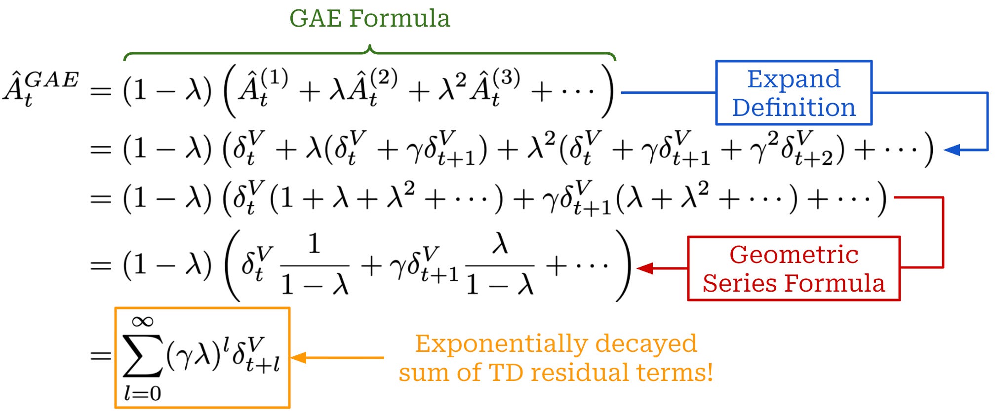
In this formulation, setting λ = 0 yields a single-step TD residual because only the first term in the sum receives a non-zero weight. Additionally, a setting of λ = 1 recovers the MC estimate. To see this, we can expand the definition of each TD residual in the sum, yielding the difference in cumulative discounted rewards and the value function of the current state V(s_t); see below.

The benefit of GAE is that the value of λ ∈ [0, 1] controls the bias variance tradeoff. As we increase the value of λ, more exact reward information is used in the advantage estimate, thus lowering the bias (but increasing variance). Similarly, we can use lower values of λ to reduce variance at the cost of higher bias.

Outcome rewards. When we are working with LLMs, we usually use an outcome reward setup, which simplifies GAE. The reward is always zero15, unless we are at the final step of the trajectory. In this scenario, most of the TD residual terms in our GAE summation are simply the difference in (discounted) value functions between two time steps γV(s_{t + 1}) - V(s_t). The final term in the summation contains the actual outcome reward observed for the trajectory.

GAE implementation. To make the concept of GAE more concrete, let’s examine a real-world example adapted from AI2’s OpenInstruct library. The full PPO training script, available here, is a great resource for learning the details of PPO in a production-grade training setting. The GAE component of this script is shown below with some additional comments for clarity. We can efficiently compute the GAE recursion by iterating through the sequence in reverse order.

import torch

# store advantages in reverse order while iterating thru sequence
advantages_reversed = []

# iterate backward to compute GAE recursion
lastgaelam = 0
gen_length = responses.shape[1]
for t in reversed(range(gen_length)):
    if t < gen_length - 1:
        # get value model prediction for time t + 1
        nextvalues = values[:, t + 1]
    else:
        # no values predicted beyond end of sequence
        nextvalues = 0.0

    # compute TD residual at time t    
    delta = rewards[:, t] + gamma * nextvalues - values[:, t]

    # add to the discounted sum of TD residuals for GAE    
    lastgaelam = delta + gamma * lam * lastgaelam

    # store the advantage for step t in our list
    advantages_reversed.append(lastgaelam)

# put the list of advantages in the correct order
advantages = torch.stack(advantages_reversed[::-1], axis=1)

Using PPO for LLMs

There are two different types of RL training that are commonly used to train LLMs (shown above):

Reinforcement Learning from Human Feedback (RLHF) trains the LLM using RL with rewards derived from a human preference reward model.
Reinforcement Learning with Verifiable Rewards (RLVR) trains the LLM using RL with rewards derived from rules-based or deterministic verifiers.

These RL training techniques differ mainly in how they derive the reward for training, but other details of the algorithms are mostly similar. As depicted below, they both operate by generating completions over a set of prompts, computing the reward for these completions, and using the rewards to derive a policy update—or an update to the LLM’s parameters—with an RL optimizer (e.g., PPO).

RLHF was the original form of RL explored by LLMs like InstructGPT [8], the predecessor to ChatGPT. Early research on RLHF for LLMs used PPO as the default RL optimizer, which ultimately made PPO a standard choice for training LLMs with RL. RLVR was introduced more recently, and most works in this space use GRPO as the underlying RL optimizer instead of PPO.

“PPO has been positioned as the canonical method for RLHF. However, it involves both high computational cost and sensitive hyperparameter tuning.” - from [9]

Downsides of PPO. Though it quickly became the default RL optimizer for RLHF, PPO is a complex actor-critic algorithm with high compute and memory overhead, as well as many low-level implementation complexities. The memory overhead of PPO is high because we keep four copies of the LLM in memory:

The policy.
The reference policy.
The critic.
The reward model (if we are using a reward model).

Additionally, we are updating the parameters of our critic alongside the policy itself and running inference for all of these models simultaneously, leading to high compute costs. Beyond memory and compute overhead, there are also many implementation details that we must carefully consider during PPO training:

How do we initialize the critic and reward model? What training settings should we adopt for these models?
What value of ε should we use for clipping in PPO?
Which model should we use as our reference model for the KL divergence?
How many policy updates should we perform for a batch of data?
Do we add the KL divergence as a penalty to the loss or directly incorporate it into the reward function? What scaling factor β should we use?
How should we weight the critic’s loss relative to the main PPO loss?
Should we use GAE? What setting should we use for λ?

Each of these choices may impact the results of RL training! PPO is a sensitive algorithm that is prone to instability—we may spend a lot of compute and time on training a model that ultimately performs poorly due to an incorrect hyperparameter setting. For these reasons, simpler RL algorithms like REINFORCE and GRPO—or even RL-free techniques like DPO—have become popular alternatives to PPO.

PPO for LLMs. In this final section, we will take what we have learned and study PPO specifically in the context of LLM training. We will focus particularly on the foundational works that were the first to use PPO for training LLMs [5, 8]—this research laid the groundwork for the modern LLM boom shortly after. While studying these papers, we will emphasize implementation details and practical lessons that are necessary to obtain a working PPO implementation.

Learning to Summarize from Human Feedback [5]

Abstractive summarization—or using models to create a human-readable, concise summary of a piece of text—has been studied for a long time. Prior to the rise of LLMs and RLHF, most papers on this topic trained language models using a supervised learning approach with human-written reference summaries and evaluated these models using traditional metrics like the ROUGE score.

These approaches can work well, but supervised learning and ROUGE are both proxies for what is actually desired—a model that writes high-quality summaries. In [5], authors solve this problem by replacing supervised learning with RLHF. Such an approach allows us to finetune language models to produce better summaries by directly using human feedback on model outputs as a training signal.

PPO for summarization. Authors in [5] are commonly credited with proposing the first RLHF framework for LLM finetuning. The proposed approach allows us to optimize an LLM based on the quality of its responses, as assessed by human annotators. Beginning with a pretrained LLM, we can iteratively:

Collect human preference data.
Train a reward model over this preference data.
Finetune our LLM with RL using this reward model.

Notably, authors in [5] adopt PPO as their underlying RL optimizer, which led PPO to become the common choice in subsequent RLHF research. With this RL training strategy, we can train an LLM to produce summaries that surpass the quality of human summaries and are even better than those produced by larger LLMs trained with a supervised learning approach; see below.

SFT stage. In [5], the LLM is first trained using supervised finetuning over human reference summaries for a single epoch, producing a supervised baseline that is later finetuned via RLHF. The methodology for RLHF proposed in [5]—as illustrated in the figure shown below—is tailored to the summarization task.

Preferences and reward models. In [5], a preference dataset is constructed by:

Grabbing a textual input to summarize—this is our prompt.
Producing many summaries of the input using several different policies—these are different responses to the same prompt.
Sampling two summaries or responses for the prompt.
Asking a human annotator to identify the better of the two summaries.

Authors in [5] collect this preference data in large batches. Once we have finished collecting a new batch of preference data, we train a reward model on the data such that it accurately predicts human preference scores given an LLM-generated summary. Then, we use this reward model to finetune our policy with PPO.

A KL divergence term is used for PPO in [5] to minimize divergence from the SFT model. Interestingly, authors in [5] were not the first to use this strategy—it was actually adopted from prior work. The KL divergence is directly subtracted from the rewards instead of being added to the PPO loss as a penalty term. We see in [5] that adding the KL divergence into RL training helps to prevent the model’s summaries from becoming too different from those seen during training.

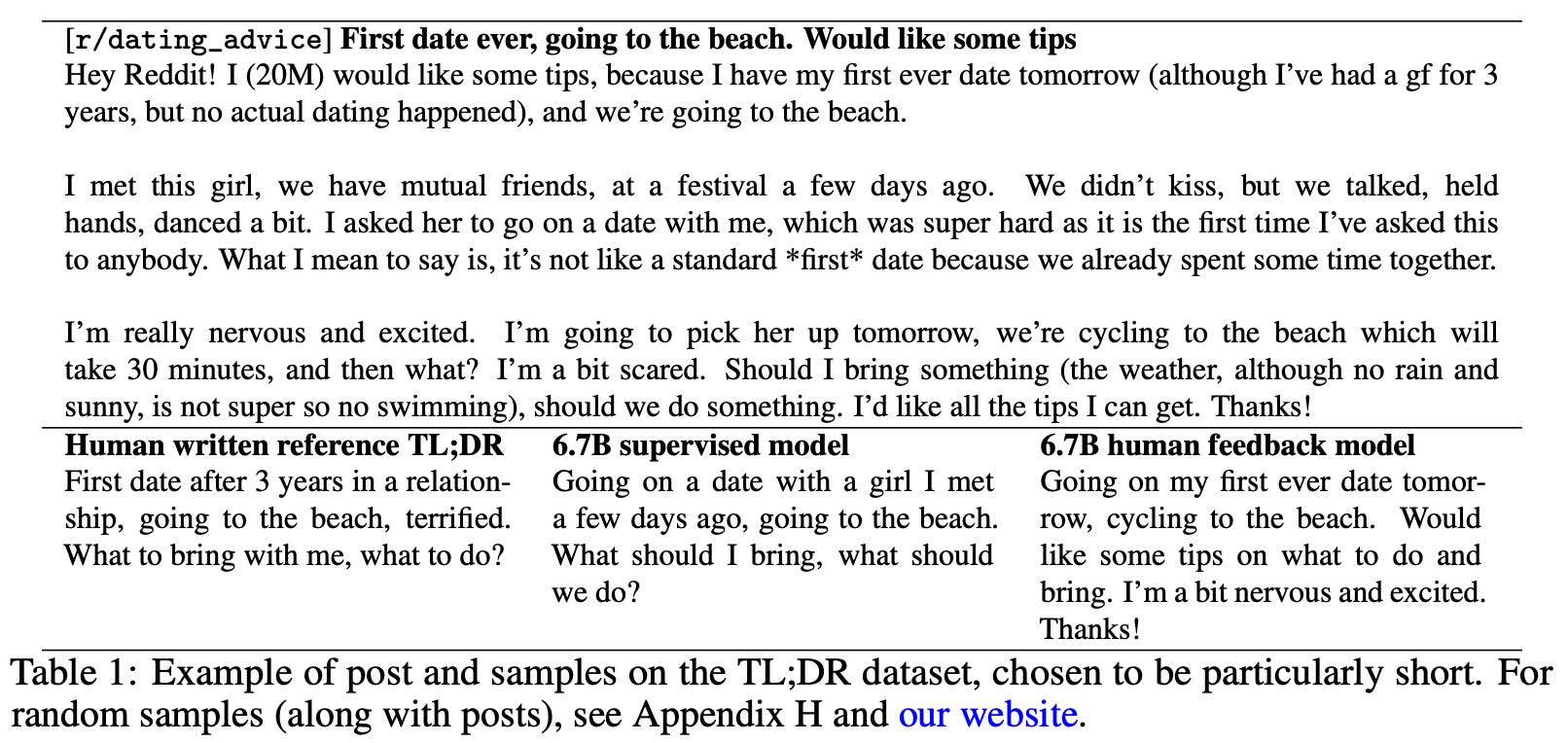
Experiments. In [5], large pretrained models matching the style of GPT-3 with 1.3B to 6.7B parameters are finetuned over the TL;DR dataset. This dataset, which contains over three million posts from Reddit with author-written summaries, is filtered to only 120K high-quality examples; see above. Models are first trained using SFT—these supervised models are also used as baselines across experiments—and then further finetuned with RLHF. Given that summary length can impact the resulting quality score, the authors in [5] constrain generated summaries to 48 tokens and finetune the model accordingly.

Finetuning language models with human feedback outperforms a variety of strong English summarization baselines. Notably, the 1.3B summarization model outperforms a 10× larger model trained with SFT, and the 6.7B summarization model performs even better than the 1.3B model, revealing that summarization quality improves with model scale. Furthermore, we see that summarization models trained via RLHF generalize better to new domains. In particular, the models in [5] are applied to summarizing news articles—a domain outside of the training data—and found to perform well without further finetuning; see below.

From here, summarization models are evaluated in terms of:

Coverage: the summary covers all information from the original post.
Accuracy: statements in the summary are accurate.
Coherence: the summary is easy to read on its own.
Quality: the overall quality of the summary is good.

When evaluated in this manner, we see that summarization models trained via RLHF benefit the most in terms of coverage, while coherence and accuracy are only slightly improved compared to supervised baseline models; see below.

Beyond summarization. Although RLHF was explored only in the context of summarization in [5], the authors of this paper had an incredible amount of foresight about what was to come. The approach proposed in [5] later became a standard part of LLM post-training, as we will soon see with InstructGPT [8].

“The methods we present in this paper are motivated in part by longer-term concerns about the misalignment of AI systems with what humans want them to do. When misaligned summarization models make up facts, their mistakes are fairly low-risk and easy to spot. However, as AI systems become more powerful and are given increasingly important tasks, the mistakes they make will likely become more subtle and safety-critical, making this an important area for further research.” - from [1]

Interestingly, authors in [5] explicitly state their intent to leverage the proposed methodology to better align LLMs to human desires in the long term. This statement was made over two years prior to the proposal of ChatGPT! Work in [5] was a building block for major advancements in AI that were yet to come.

The N+ Implementation Details of RLHF with PPO [4]

There are many moving parts in PPO training, including multiple copies of the LLM (i.e., policy, reference, critic, and reward model) and various hyperparameter settings that must be carefully tuned to ensure stable training. For these reasons—and due to computational expense—reproducing RL training results is difficult.

“It has proven challenging to reproduce OpenAI’s RLHF pipeline… for several reasons: 1) RL and RLHF have many subtle implementation details that can significantly impact training stability, 2) the models are challenging to evaluate… 3) they take a long time to train and iterate.” - from [4]

As a starting point for democratizing understanding of RL, authors in [4] focus on a simple setup—OpenAI’s prior work on RLHF for summarization [5]. Though many details are already provided in the original work, authors in [4] fully reproduce these results while enumerating all implementation details needed to arrive at a working PPO implementation. The TL;DR summarization task is simple relative to most modern RLHF pipelines. However, this study—based on Pythia models [10] with 1B, 2.8B, and 6.8B parameters—provides a clear and comprehensive view of key practical considerations when training an LLM with PPO.

Dataset considerations. Authors in [4] enumerate around 20 practical details needed to obtain a working RLHF pipeline with PPO. Nearly half of these details are not related to PPO—they focus on the training data. For those who have worked with LLMs, this data emphasis should not come as a surprise: data quality is the key determinant of success in all forms of LLM training, including RL.

All experiments in [4] use the TL;DR summarization dataset from OpenAI, which contains both an SFT and preference dataset. Some notable remarks about the data used for PPO in [4] include:

There is a misalignment in completion lengths between the SFT and preference portion of the TL;DR dataset—the preference data tends to have longer completions.
Data must occasionally be truncated to fit within the fixed sequence length used in [4], but the authors choose to truncate at paragraph boundaries—determined by newline characters—instead of performing a hard truncation at the maximum sequence length.
All completions are followed by an <EOS> token. Authors in [4] emphasize that this <EOS> token must be different than the padding token used by the LLM. Otherwise, the loss for the <EOS> token will be masked with the other padding tokens, preventing the model from learning to properly complete each sequence with an <EOS> token.

Reward model. Several choices exist for initializing the reward model in RLHF. In [4], we initialize with the weights of the SFT model, which matches settings used in [5]. A randomly-initialized linear head that is used to predict the reward is then added to the reward model’s architecture before the model is trained for a single epoch over the available preference data.

An outcome reward setting is used in [4]. To extract the reward, a forward pass is performed on the full sequence, and we extract the reward prediction from the <EOS> token only. To teach the policy to consistently output sequences of reasonable length with a corresponding <EOS> token, the EOS trick is used, which assigns a reward of -1 to any sequence with no <EOS> token.

“If the padding token does not exist, the extracted reward will then be logits corresponding to the last token of the sequence – if that token is not the EOS token, its reward won’t be used for PPO training” - from [4]

After the reward model is trained, authors follow the recommendation in [5] of normalizing rewards outputted by the model. Specifically, the reward model is used to predict rewards for the entire SFT dataset. Then, we compute the mean reward across this dataset and use this mean to center the average reward. In other words, this mean is subtracted as a bias from the reward model’s output, ensuring that rewards predicted over the SFT dataset have an average of zero. Normalizing the reward model’s output benefits training stability for PPO.

Critic settings. We must also choose how to initialize the critic. In [4], the critic is initialized with the weights of the reward model at the beginning of PPO training. After all, the value model is effectively a reward model that predicts the reward on a per-token basis. Authors observe in [4] that the reward model’s predictions are usually negative for all tokens except the <EOS> token; see below.

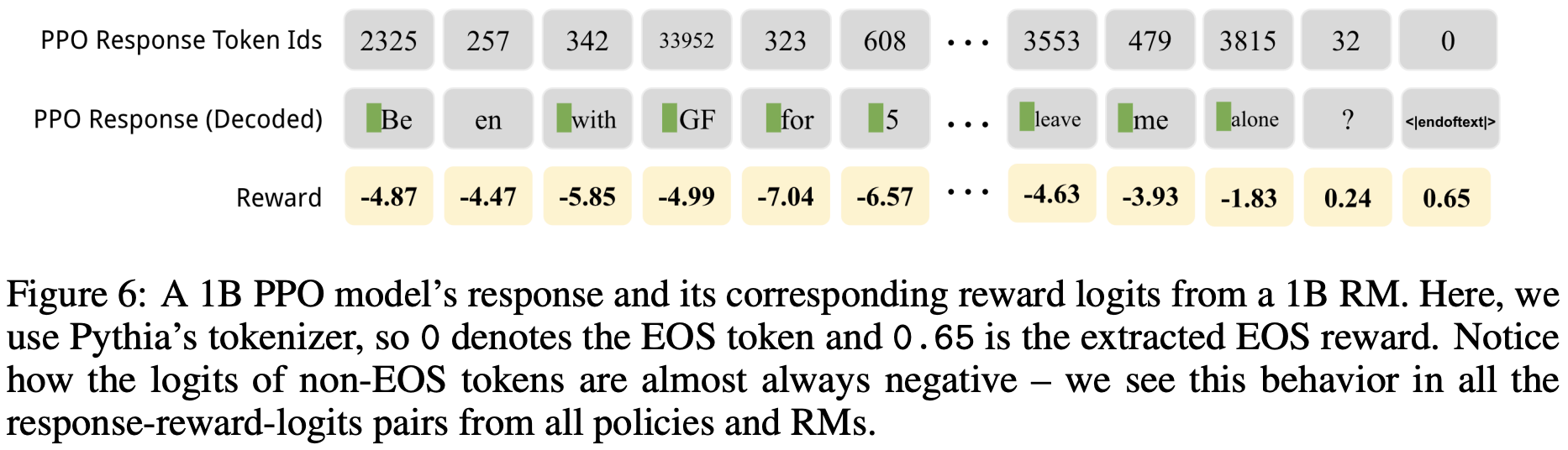
Therefore, the value estimated by the critic is negative for nearly every token at the start of PPO training. However, we see in [4] that warm starting the critic in this way helps to improve the initial stability of gradients during training.

Reward and advantage whitening. In addition to normalizing rewards after training the reward model, many PPO implementations perform reward and advantage whitening. An example implementation of the whitening operation is shown below, where the values can be a list of either rewards or advantages.

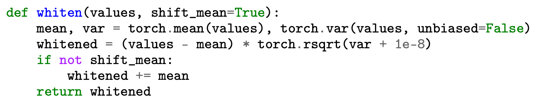
When whitening rewards, we usually do not shift the mean (i.e., shift_mean = False in the above code) so that we can retain the magnitude and sign of the rewards. However, the mean is usually shifted when whitening advantages. Based on results in [4], whitening rewards and advantages does not seem to have a huge positive or negative performance impact on the resulting policy. However, whitening is a common implementation detail in PPO. Usually, whitening is applied over the set of rewards or advantages within a batch of data.

“Where normalization bounds all the values from the RM to be between 0 and 1, which can help with learning stability, whitening the rewards or the advantage estimates… can provide an even stronger boost to stability.” - from [2]

Beware of dropout. We must also be sure to avoid using dropout in PPO. Dropout adds noise to the model’s forward pass, making the computation of policy ratios and KL divergence unreliable. This implementation detail can cause optimization issues and tends to be impactful—dropout is a perfect example of small but important practical details in PPO. For example, the OpenInstruct PPO script explicitly disables dropout in the policy, critic, reference, and reward models.

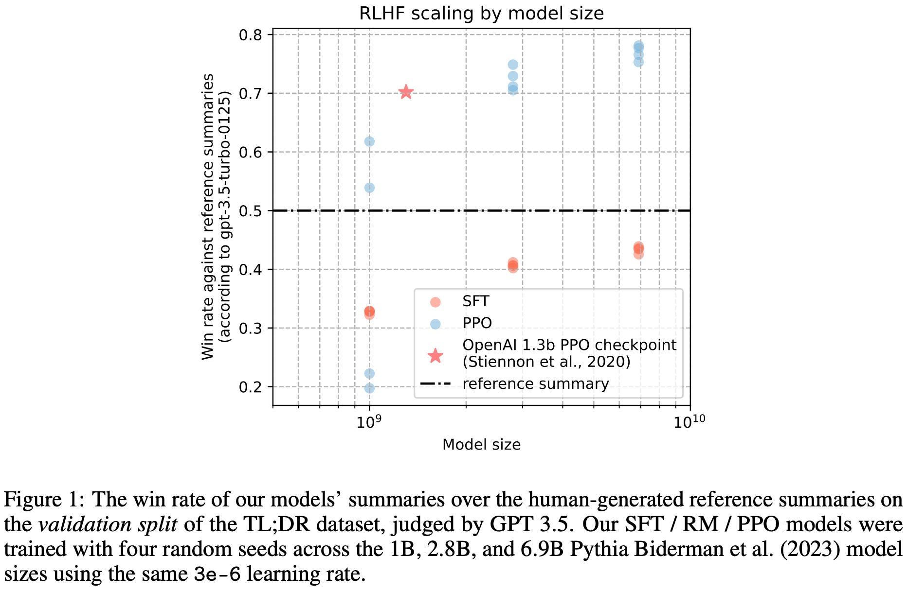
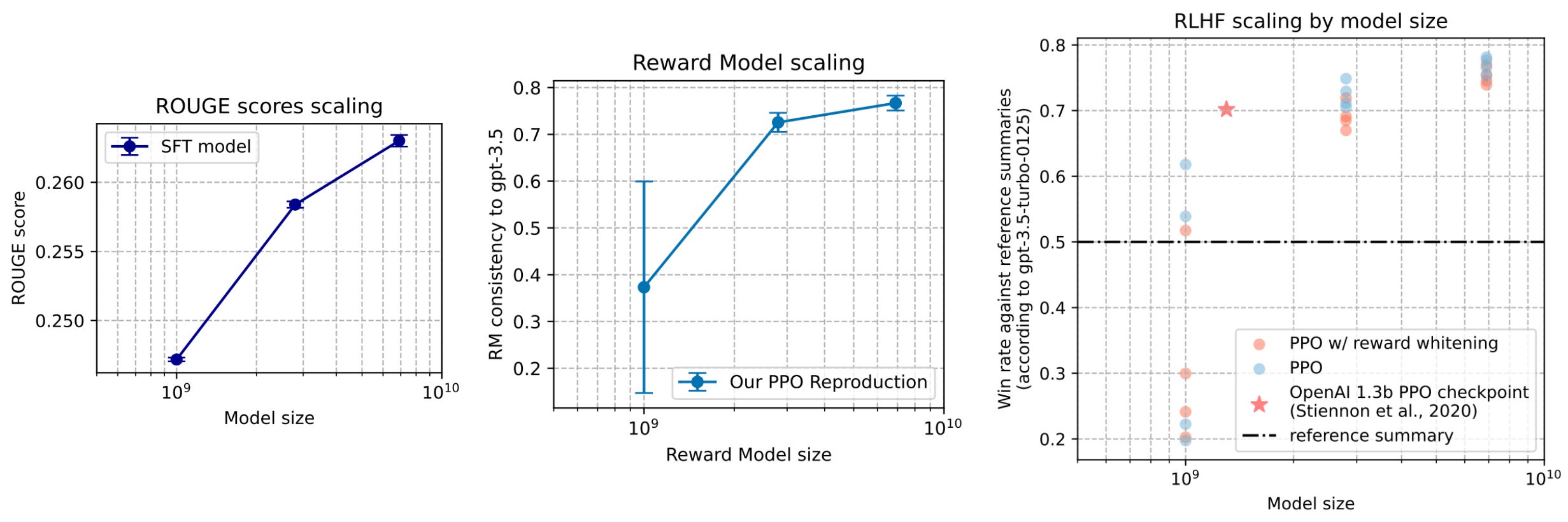
Final results. After enumerating various practical choices and hyperparameter settings, the policies in [4] successfully replicate the original results of [5]. PPO models outperform those trained with SFT, and there are clear scaling trends that can be observed (i.e., larger models achieve better performance metrics) for SFT models, reward models, and the final RL policies. Additionally, the preference rate of the RL policies over human reference summaries—as predicted by a GPT-3.5-based LLM judge—scales predictably with model size; see below.

Training language models to follow instructions with human feedback [8]

Going beyond the summarization domain, authors in [8] explore the use of RLHF for language model alignment by directly learning from human feedback. The resulting model, called InstructGPT, is the sister model and predecessor to ChatGPT. Since this model is outlined and explained in detail in [8], the work provides significant insight into how early LLMs at OpenAI were trained.

Following an approach similar to [5], we start with a set of prompts that are either written by human annotators or collected from OpenAI’s API. We can then have annotators write responses to these prompts and finetune a pretrained LLM—GPT-3 in particular—over these examples using SFT. Using this model, we can then collect comparison data by asking humans to select their preferred outputs from the LLM and apply the same RLHF process outlined in [5] for finetuning. As shown above, the resulting model is heavily preferred by humans and much better at following detailed instructions provided within the prompt.

“Making language models bigger does not inherently make them better at following a user’s intent.” - from [8]

The alignment process. Pretrained LLMs have a number of undesirable properties that we want to fix during post-training; e.g., hallucinations or an inability to follow detailed instructions. To fix these issues, we align the LLM in [8] according to the following set of criteria:

Helpful: follows the user’s instructions and infers intention from few-shot prompts or other patterns.
Honest: makes correct factual statements about the world.
Harmless: avoids harmful outputs, such as those that denigrate a protected class or contain sexual/violent content.

Using RLHF, we can teach an LLM to reflect each of these qualities within its output. Specifically, this is done by constructing preference pairs where the preferred responses are chosen based upon adherence to these criteria.

More on RLHF. Authors in [8] curate a team of 40 human annotators, who are screened with a test to judge their annotation quality, to collect preference data for the LLM. The approach for RLHF used in [8] matches the approach used in [5] almost completely. Using a pretrained LLM and a set of prompts for finetuning, the alignment process proceeds according to the following steps:

Collect human demonstrations of responses for each prompt.
Train the model in a supervised fashion over human demonstrations.
Collect preference data.
Train a reward model.
Optimize the underlying LLM or policy with PPO.
Repeat steps 3-5.

The distribution of prompts used for finetuning in [8] is outlined in the table below. For SFT, a dataset of over 13K prompt and response pairs is constructed. The reward model is trained over 33K prompts, while a dataset of size 31K is used for finetuning with PPO. Unlike [5], human annotators are shown 4-9 responses to a prompt (i.e., instead of two) when collecting comparison data, allowing them to quickly rank responses and generate larger amounts of comparison data more efficiently. However, later work on RLHF largely abandoned this approach in favor of binary preferences. The dataset used in [8] is also 96% English.

Similarly to [5], a KL divergence term between the policy and the SFT model is directly subtracted from the reward to avoid drifting too far away from the SFT model. Additionally, extra pretraining updates are “mixed in” to the RLHF optimization process, which authors find to help with maintaining the model’s performance across various benchmarks. These pretraining updates, which use a supervised loss, are simply added to the PPO loss used during RL.

“We were able to mitigate most of the performance degradations introduced by our fine-tuning. If this was not the case, these performance degradations would constitute an alignment tax—an additional cost for aligning the model.” - from [2]

Experimental findings. In [8], authors train three models with 1.3B, 6B, and 175B (i.e., same as GPT-3) parameters. From these experiments, we learn that human annotators prefer InstructGPT outputs over those of GPT-3, even for models with 10× fewer parameters; see below. This result is similar to observations in [5], where finetuning via RLHF enables much smaller models to outperform larger models trained in a supervised manner.

Notably, outputs from InstructGPT-1.3B are preferred to those of GPT-3, which has 100× more parameters. Additionally, we see that InstructGPT-175B produces outputs that are preferred to GPT-3 85% of the time. Going further, InstructGPT models are found to more reliably follow explicit constraints and instructions provided by a human user within the model’s prompt; see below.

Compared to pretrained and supervised models, InstructGPT is also found to be:

More truthful.
Slightly less toxic.
Generalizable to instructions beyond the training dataset.

For example, InstructGPT can answer questions about code and handle prompts written in different languages, despite the finetuning dataset lacking sufficient data within this distribution. Although the model did not receive as much recognition as ChatGPT, InstructGPT was a major step forward in AI that introduced many core concepts used for training modern LLMs.

Conclusion

PPO is one of the most widely used RL algorithms for LLMs that has—through its key role in RLHF pipelines—directly contributed to fundamental advancements in AI. As we learned, research on PPO was an important factor in the creation of models like InstructGPT and ChatGPT. These influential models catalyzed the ongoing boom in LLM research in which we currently find ourselves.

We cannot overstate the impact of PPO on LLM research, and PPO continues to play an important role in LLM post-training pipelines today. However, the barrier to entry for PPO is high due to its memory and compute overhead. Additionally, the results of PPO can vary based on a wide variety of practical implementation details and hyperparameter settings. For these reasons, most research on PPO has been centralized within top frontier labs. Only a small number of groups have sufficient compute resources to empirically tune and obtain a working PPO implementation at scale.

Nonetheless, understanding PPO is essential due to its fundamental role in AI research. The cost and complexity of PPO remains high, but RL researchers have recently expanded and improved upon ideas proposed by PPO. For example, REINFORCE and GRPO are simpler (and more stable) policy gradient algorithms that can be used to train LLMs, which use less memory than PPO by avoiding the critic. A working understanding of PPO makes understanding these new algorithms—or even developing our own—much simpler!

New to the newsletter?

Hi! I’m Cameron R. Wolfe, Deep Learning Ph.D. and Senior Research Scientist at Netflix. This is the Deep (Learning) Focus newsletter, where I help readers better understand important topics in AI research. The newsletter will always be free and open to read. If you like the newsletter, please subscribe, consider a paid subscription, share it, or follow me on X and LinkedIn!

Bibliography

[1] Schulman, John, et al. “Proximal policy optimization algorithms.” arXiv preprint arXiv:1707.06347 (2017).

[2] Lambert, Nathan. “Reinforcement Learning from Human Feedback.” Online (2025). https://rlhfbook.com

[3] Schulman, John, et al. “High-dimensional continuous control using generalized advantage estimation.” arXiv preprint arXiv:1506.02438 (2015).

[4] Huang, Shengyi, et al. “The n+ implementation details of rlhf with ppo: A case study on tl; dr summarization.” arXiv preprint arXiv:2403.17031 (2024).

[5] Stiennon, Nisan, et al. “Learning to summarize with human feedback.” Advances in neural information processing systems 33 (2020): 3008-3021.

[6] Schulman, John, et al. “Trust region policy optimization.” International conference on machine learning. PMLR, 2015.

[7] Lambert, Nathan, et al. “Tulu 3: Pushing frontiers in open language model post-training.” arXiv preprint arXiv:2411.15124 (2024).

[8] Ouyang, Long, et al. “Training language models to follow instructions with human feedback.” Advances in neural information processing systems 35 (2022): 27730-27744.

[9] Ahmadian, Arash, et al. “Back to basics: Revisiting reinforce style optimization for learning from human feedback in llms.” arXiv preprint arXiv:2402.14740 (2024).

[10] Biderman, Stella, et al. “Pythia: A suite for analyzing large language models across training and scaling.” International Conference on Machine Learning. PMLR, 2023.

As we can see, the discounted reward has an infinite horizon in this case. In other words, the total number of steps in the trajectory is infinite T = ∞. This is known as the infinite-horizon discounted return.

The VPG was also partially covered in my overview of REINFORCE that was released a few weeks ago; see here.

Specifically, if we wanted to solve a constrained optimization problem like this with gradient ascent, we would have to use constrained gradient ascent. However, this method requires that we project our solution into the space of valid solutions that satisfy the constraint after every optimization step, which would be computationally intractable for neural network parameters. The KL divergence is a very complex constraint for which to perform this projection!

More specifically, if the policy ratio is greater than 1 + ε, we set it equal to 1 + ε. If the policy ratio is less than 1 - ε, we set it to 1 - ε. Otherwise, we keep the value of the policy ratio unchanged.

The clipped objective will always be less than or equal to the unclipped objective due to the fact that we are taking the minimum of the unclipped and clipped objectives.

The “actor” refers to the LLM—or the model that is taking actions—and the “critic” refers to the value model. The value model is called a critic due to the fact that it is predicting the reward associated with each action (i.e., effectively critiquing the action).

For more details on loss aggregation in RL, see this section of the RLHF book, which provides concrete examples of different aggregation strategies and their impact.

The adaptive KL divergence is explained in Section 4 of [1]. Instead of setting a fixed scaling factor for the KL divergence, authors propose dynamically adjusting this factor throughout training such that the KL divergence stays close to a target KL divergence d_targ. Put differently, instead of choosing the scaling factor, we specify what we want our KL divergence to be and dynamically adjust the scaling factor throughout training to keep the KL divergence in this range. This approach is not commonly used for recent LLMs, and it is much more common to set a fixed β coefficient for the KL divergence.

The reference and old models are different models in PPO! The reference model is the policy parameters before any RL training is performed. For LLMs, the SFT model is usually the reference model. We usually perform multiple updates over a batch of data in PPO, and the old model is the model before the first update. The old model is updated each time a new batch of data is sampled, whereas the reference model is fixed.

This means that less data is required to achieve a given level of performance (i.e., the learning process is faster).

Specifically, we would use the cumulative reward after state s_t. However, for LLMs this distinction does not usually matter due to the use of outcome rewards.

In fact, this is where the name for the TD residual comes from. We are computing the difference in value between two time steps.

The critic is just a model that imperfectly estimates of the value function. The bias in the TD residual comes from the fact that the critic makes mistakes in estimating the value.

To derive this expression, we begin with the original formula for the GAE showed in the top line, expand the definitions of the N-step advantage estimates, rearrange the terms, then use the geometric series formula to derive the final expression.

This statement assumes that the KL divergence is added to the loss and not directly incorporated into the reward.

NEOCLOUD DEEP DIVES

17h

This comprehensive guide brilliantly bridges the gap between theoretical RL and practical LLM implementation. The progression from basic policy gradients to GAE is particularly well structred. Your breakdown of the four clipping cases in PPO finally made that mechanism click for me - seeing how advantage sign determines when clipping activates is invaluable.

Expand full comment

1 reply by Cameron R. Wolfe, Ph.D.

1 more comment...

Deep (Learning) Focus