
Direct Preference Optimization (DPO)
How to align LLMs with limited hardware and minimal complexity...

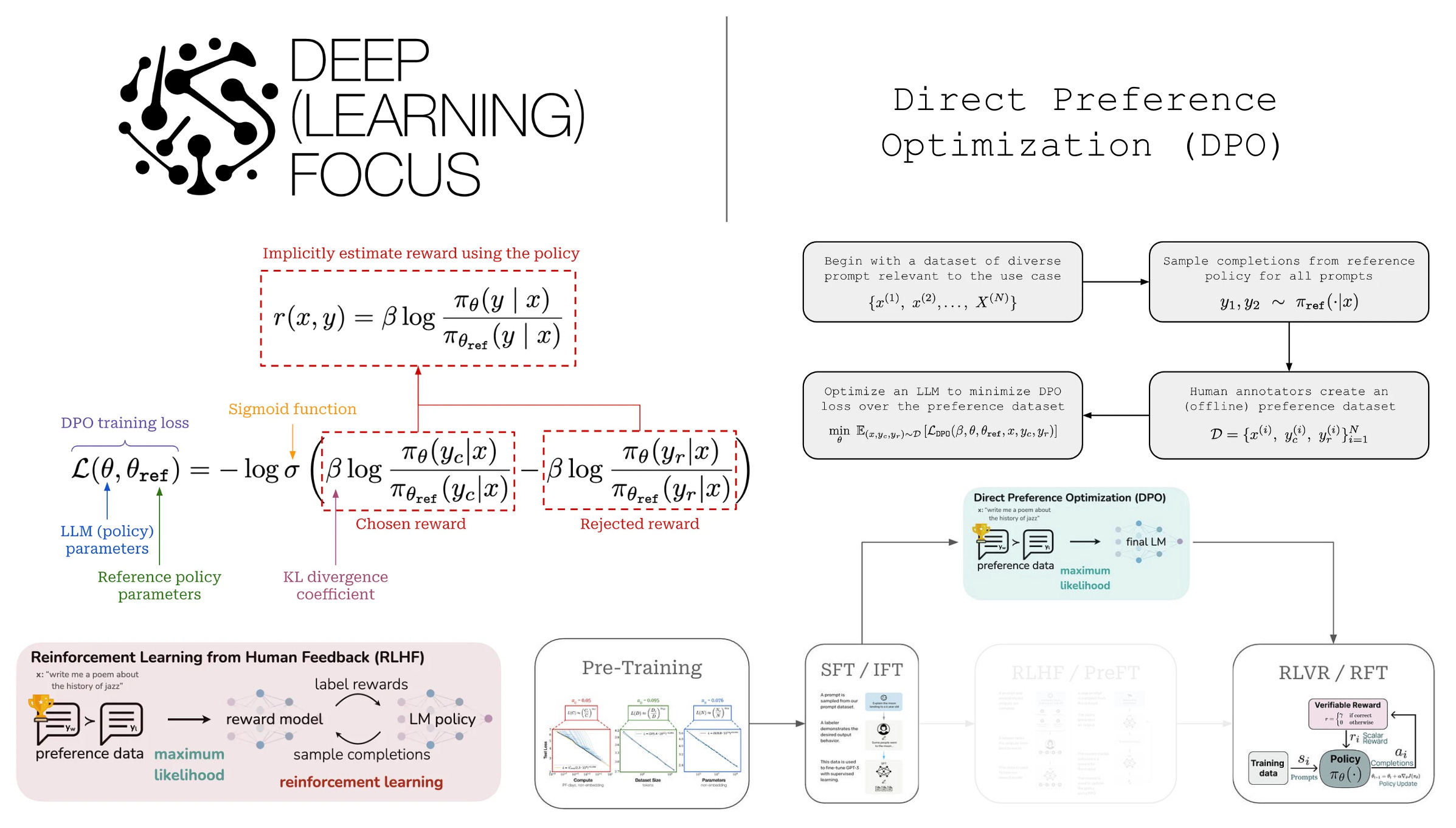
Aligning large language models (LLMs) is a crucial post-training step that ensures models generate responses aligned with human preferences. While alignment techniques like reinforcement learning from human feedback (RLHF) led to massive improvements in LLM quality, they are complex, computationally expensive, and challenging to optimize. In this overview, we will learn about a simpler approach to LLM alignment, called Direct Preference Optimization (DPO), that avoids these complexities by aligning LLMs with a simpler objective that can be optimized with gradient descent. The performance and practicality of DPO makes alignment research more accessible and have allowed it to become a standard post-training algorithm that is actively used by several popular LLMs.
“Direct alignment algorithms allow one to update models to solve the same RLHF objective without ever training an intermediate reward model or using reinforcement learning optimizers. The most prominent direct alignment algorithm and one that catalyzed an entire academic movement of aligning language models is Direct Preference Optimization (DPO).” - RLHF book
The Building Blocks of DPO
To fully understand DPO, we first need to lay the groundwork for this technique by understanding how LLMs are trained. Specifically, DPO is a preference tuning algorithm that is used in the LLM post-training process. This algorithm finetunes the LLM over a human preference dataset and is an alternative to RL-based preference tuning techniques like (PPO-based) RLHF. In this section, we will discuss these ideas to contextualize DPO and its role in LLM training.
Preference Data and Reward Models
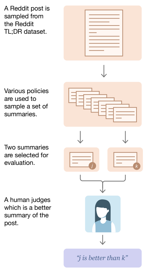
Human preferences are a pivotal component of the LLM post-training process. Preference data usually has the above form, where we have a single prompt, two responses (or completions) to this prompt, and a preference—assigned either by a human annotator or an LLM judge—for these completions. The preference simply indicates which of the two responses is better than the other.
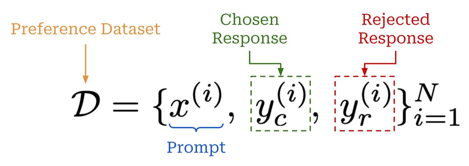
This concept is formalized via the expression above, which defines a preference dataset of prompts with an associated “chosen” and “rejected” response.
The Bradley-Terry Model of Preference is the most popular statistical model to use for modeling preferences within the LLM domain. At a high-level, Bradley-Terry takes two items (e.g., a chosen and rejected completion) and an associated reward for each of these items as input. Using this information, we can express the probability that one item is preferred over another as shown below. Here, we assume that the items we are comparing are structured as a preference pair.
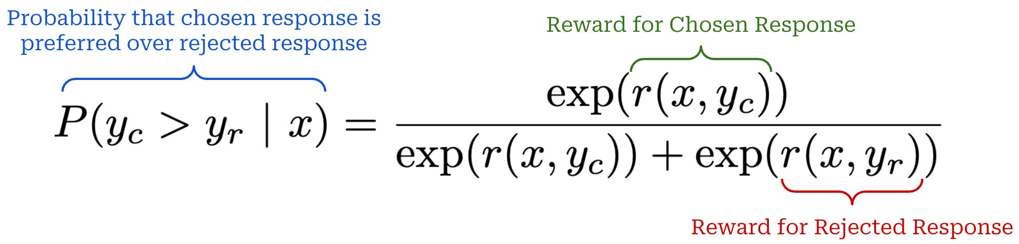
We use the Bradley-Terry model to express probabilities for pairwise comparisons between two completions. However, Bradley-Terry is not the only approach that we can use to model preferences; e.g., the Plackett-Luce model is another option.
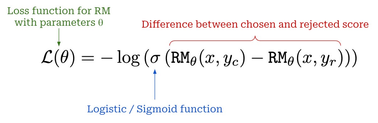
Reward Models. The reward in the expression above is usually predicted by a reward model (RM). An RM is a specialized LLM—implemented by adding an extra linear classification head to the standard decoder-only transformer (shown below)—that takes a prompt-completion pair as input and outputs a (scalar) preference score.

Given a fixed preference dataset, we can train an RM to produce scores that reflect the observed human preferences, as modeled by Bradley-Terry. In other words, we want to maximize the probability that chosen responses are preferred to rejected responses—given by the pairwise probability expression above—by our RM across the preference dataset. To do this, we can simply minimize the negative log-likelihood loss shown below using maximum likelihood estimation (MLE)—this means we train our RM over many data examples using this objective as our loss function. For further details on RMs, please see the overview linked below.

LLM Training & Alignment
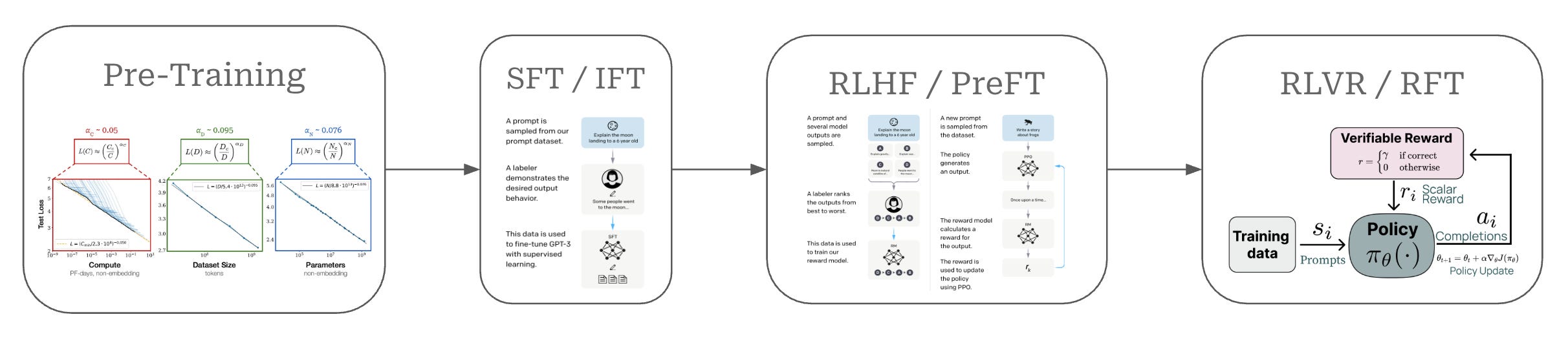
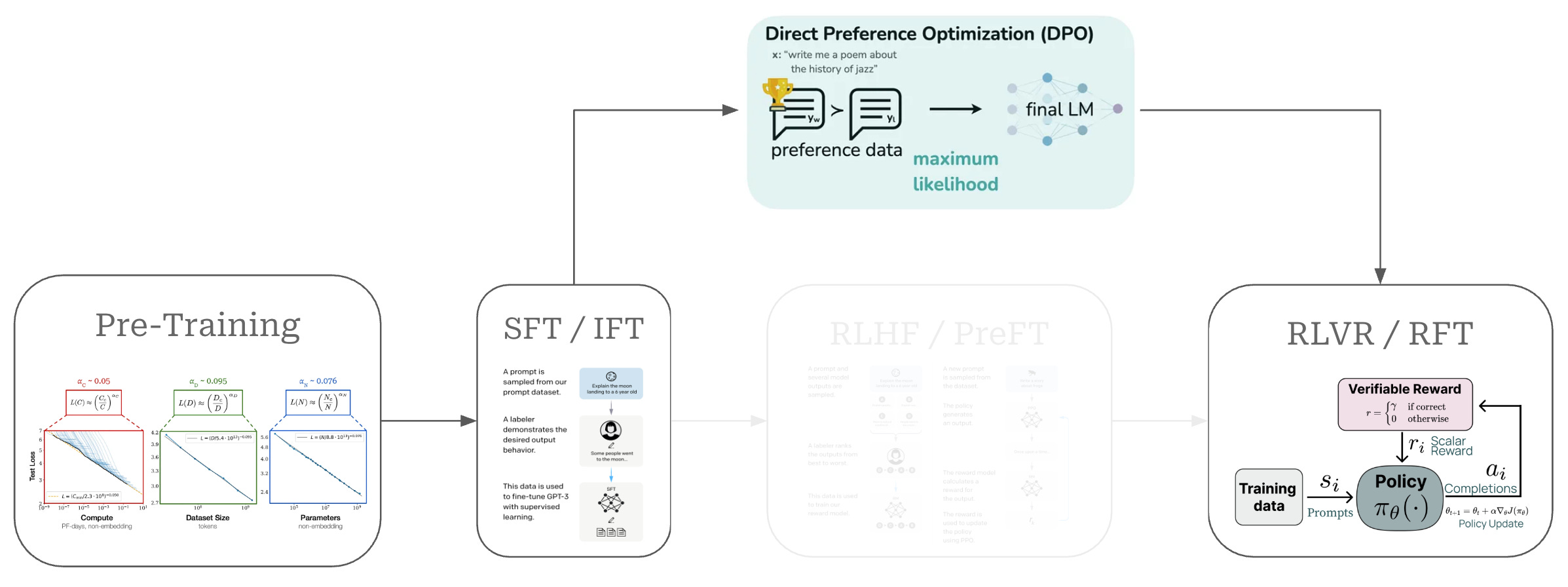
Given that this overview will focus upon DPO, we need to understand where DPO fits into the overall training process for an LLM. This training process, which has (roughly) four parts, is depicted in the figure above. We can break down each of these steps and their corresponding purpose as follows:
Pretraining is a large-scale training procedure that trains the LLM from scratch over internet-scale text data using a next token prediction training objective. The primary purpose of pretraining is to instill a broad and high-quality knowledge base within the LLM; see here.
Supervised finetuning (SFT) or instruction finetuning (IFT) also uses a (supervised) next token prediction training objective to train the LLM over a smaller set of high-quality completions that it learns to emulate. The primary purpose of SFT is to teach the LLM basic formatting and instruction following capabilities; see here.
Reinforcement learning from human feedback (RLHF) or preference finetuning (PreFT) uses reinforcement learning (RL) to train the LLM over human preference data. The key purpose of RLHF is to align the LLM with human preferences; i.e., teach the LLM to generate outputs that are rated positively by humans as described here.
Reinforcement learning from verifiable rewards (RLVR) or reinforcement finetuning (RFT) trains the LLM with RL on verifiable tasks, where a reward can be derived deterministically from rules or heuristics. This final training stage is useful for improving reasoning performance or—more generally—performance on any verifiable task.
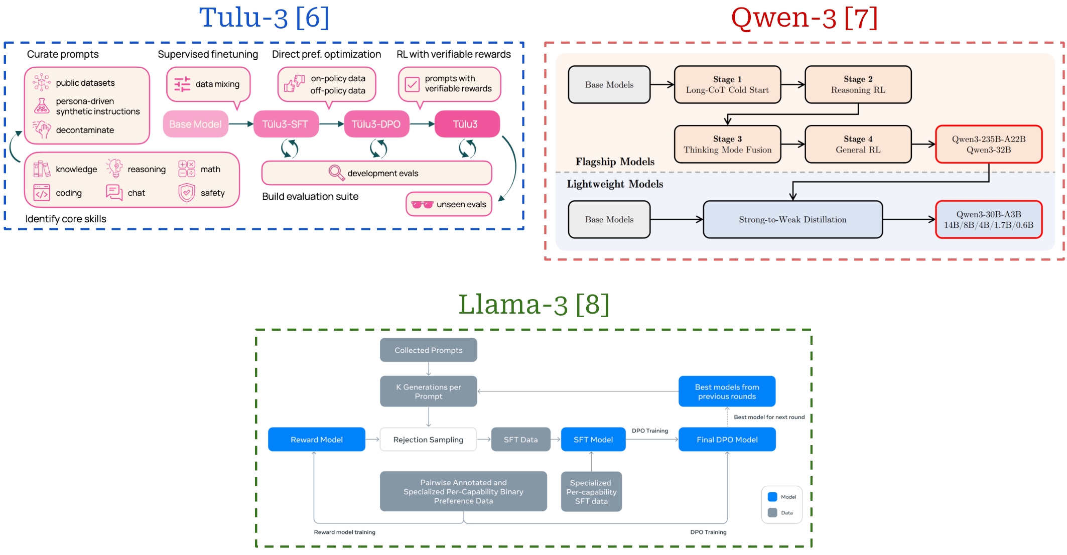
As we can see, each of these training stages play a key purpose in the process of creating a high-quality LLM. These training techniques can be grouped into the broad categories of pretraining and post-training—or everything that comes after pretraining. Pretraining is always the first step of training an LLM, but the post-training process can vary widely depending on the LLM being trained. The same techniques—i.e., SFT, RLHF and RLVR—are usually used, but their exact ordering and setup can change. See the image below for several examples of LLM post-training pipelines that each adopt a slightly different setup.
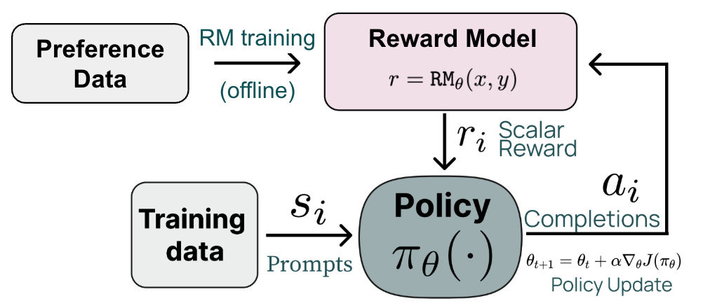
More on RLHF. All of the LLM training stages are important, but this overview will focus on the RLHF stage in particular, which is responsible for aligning the underlying LLM to human preferences. The RLHF training process has three major steps (shown below):
Collect a human preference dataset that captures preferable behaviors we want to instill into the LLM.
Train a separate reward model (RM) over this preference dataset.
Finetune the LLM with RL1 using the output of the RM as the reward.
The third step of this process usually happens in an online fashion, meaning that we are generating completions from our policy to be scored by the RM during the training process2. Online RL training is difficult to setup and orchestrate efficiently [10].
Many RL-based optimizers exist (e.g., PPO, REINFORCE, GRPO and more) that could be used to power the third stage of RLHF. However, the standard choice—as originally popularized by [2]—of RL optimizer for RLHF is Proximal Policy Optimization (PPO). PPO-based RLHF is a common choice in top LLM labs and tends to yield the best results in large-scale LLM post-training runs.
“While RLHF produces models with impressive conversational and coding abilities, the RLHF pipeline is considerably more complex than supervised learning, involving training multiple LMs and sampling from the LM policy in the loop of training, incurring significant computational costs.” - from [1]
Despite its effectiveness, PPO has several downsides. In addition to being an online RL algorithm, PPO stores four different copies of the LLM (i.e., policy, reference policy, reward model and value function) in memory, which means that we need many GPUs with lots of memory available to perform training with PPO. Additionally, a litany of implementation details are present in PPO-based RLHF that—if not tuned properly—can result in sub-optimal performance.
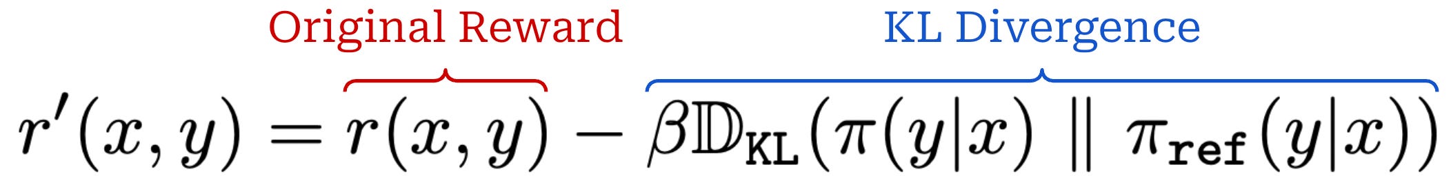
What happens during RL training? During the RL training step of RLHF, we have a learned reward model available, and we want to maximize the rewards assigned by this reward model to our LLM’s outputs. Additionally, we want to avoid “drifting” too far away from our original model during training. This optimization process is usually formulated via the objective shown below.
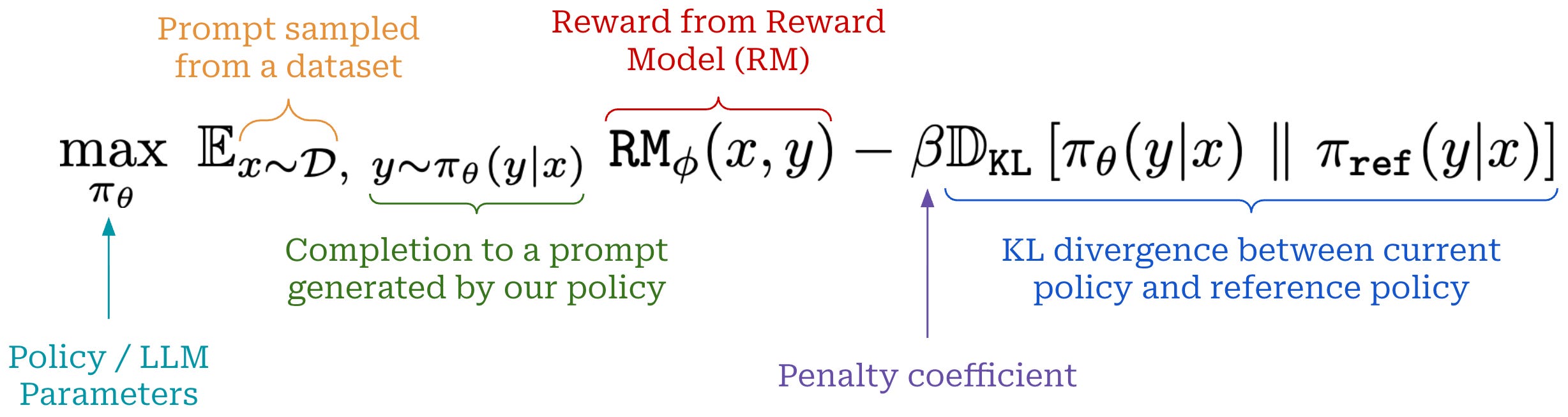
In this equation, we maximize the expected reward received by our LLM’s completions under an additive penalty for the KL divergence between the learned policy and the initial SFT model (or any other reference model)—the KL divergence is included as a penalty term in the loss function. The tradeoff between the reward and KL divergence is controlled by the hyperparameter β.
Why is RLHF so hard? RL-based preference tuning is complex to use for a variety of reasons; e.g., multiple LLMs are involved, generations must be sampled from these models during training, hyperparameter tuning is required and the compute / memory costs are high. In practice, these complexities make the RLHF training process unstable, unpredictable, expensive and generally difficult. These issues significantly raise the barrier to entry for doing research on LLM post-training.
At a high level, there are two key reasons that PPO-based RLHF is so complex, expensive and difficult to implement properly:
Using an explicit reward model.
Using RL to train the LLM.
The reward model is an additional LLM that we must train separately and store in memory during training. Additionally, the use of PPO for training introduces another copy of the model—the value function—that we must store in memory, as well as all the addition difficulties of RL-based preference tuning. Therefore, if we could simply avoid the separate reward model and the use of RL, many of the common headaches associated with PPO-based RLHF would be avoided as well!
Where does DPO fit in? As shown above, DPO is an alignment algorithm that serves as an alternative to RLHF. Unlike RLHF, however, DPO optimizes the policy via gradient ascent to solve the RLHF objective in an indirect manner, without using a separate reward model or any form of RL training.
“We show how to directly optimize a language model to adhere to human preferences, without explicit reward modeling or reinforcement learning. We propose DPO, an algorithm that implicitly optimizes the same objective as existing RLHF algorithms but is simple to implement and straightforward to train.” - from [1]
DPO addresses the RLHF objective by introducing a novel reparameterization of the reward, deriving it directly from the policy rather than from a separate reward model—this is referred to as an “implicit” reward. When training LLMs with DPO, we learn this implicit reward using an offline preference dataset in a manner similar to training a conventional reward model. The key insight of DPO is that we can extract the optimal policy for RLHF directly from this implicit reward. Fundamentally, DPO learns an implicit reward model—grounded in the Bradley-Terry model—and indirectly derives the optimal policy from this implicit reward.
Because DPO does not require training a separate, explicit reward model, some practitioners mistakenly believe that DPO “avoids” reward modeling altogether and directly optimizes the policy via RLHF without any RL or reward model. In reality, DPO is still a reward modeling approach: its training objective and process are identical to those of traditional reward modeling. In DPO, we are indeed training a reward model—the only difference is that this reward model is implicit within the policy itself. By training our policy to optimize this implicit reward, DPO enables us to find a policy that optimally solves the RLHF objective as well.
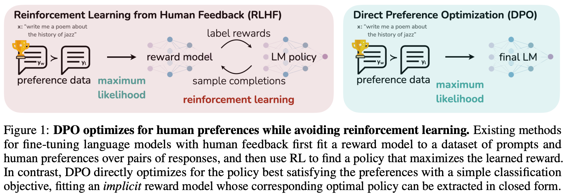
As depicted above, DPO avoids external reward models, online sampling, and RL as a whole. Instead, we directly optimize the LLM using basic gradient descent to (implicitly) solve the RLHF objective. These simplifications make DPO more stable—requiring less hyperparameter tuning—and lightweight compared to RL-based preference tuning, which helps to democratize post-training research.
Kullback-Leibler (KL) Divergence
Throughout LLM post-training, there are many cases where we optimize our model subject to a KL divergence constraint. For example, the canonical optimization objective used within RLHF has the form shown below.
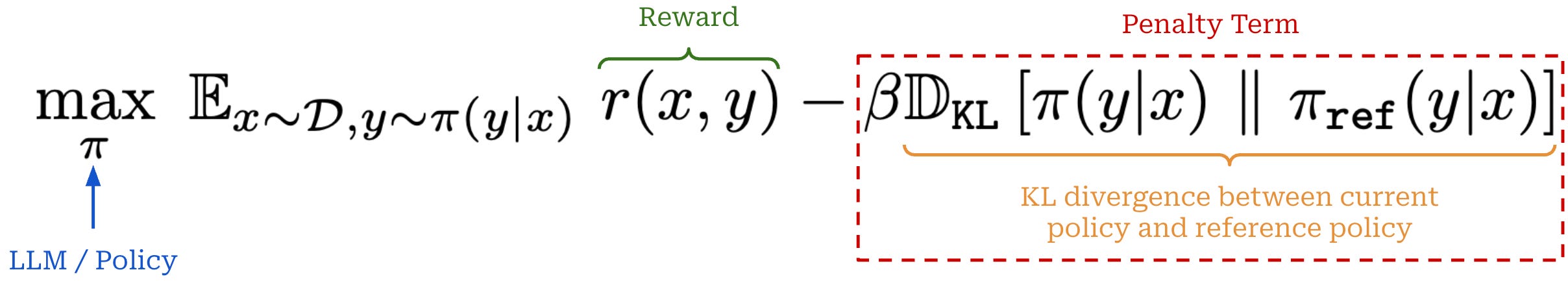
As we can see, we want to maximize rewards while minimizing a penalty term—the KL divergence weighted by β—that is subtracted from these rewards. The goal of the penalty term is to avoid our policy3 drifting too far away from a reference policy during training. Let’s dive deeper to understand exactly what this means.
KL divergence is a concept from information theory that measures how different4 a probability distribution is from some reference distribution. For a discrete probability distribution, the KL divergence has the form shown below. Notably, KL divergence is not symmetric—the order of arguments matters.

In the case of a continuous probability distribution, we can formulate the KL divergence as an expectation; see above. If this concept is not clear, read this.
Relation to LLMs. In the LLM domain, KL divergence is commonly used to compare two LLMs or policies. Typically, we will compare the policy that we are currently trying to train to a reference policy. For example, in the case of DPO, we begin with an SFT policy (i.e., an LLM that has already undergone both pretraining and SFT), then optimize the standard RLHF objective, where the KL divergence is computed between this SFT (reference) policy and the policy that we are training. Specifically, the form of this KL divergence would be:
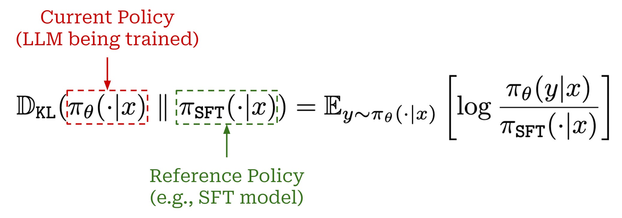
This form of the KL divergence looks at the ratio of probabilities predicted by both the current and reference model for a completion y given a prompt x as input. The probability of a completion y is simply the product of next token probabilities predicted by the LLM for each token within a completion. By computing the KL divergence over these completion probabilities, we capture the similarity between the token distributions predicted by the two models.
Estimating KL divergence in practice. We usually want to estimate the KL divergence between distributions predicted by our current policy and a fixed reference policy (e.g., the SFT model5) during RL training. Intuitively, adding this constraint to the reward used during RL training (as shown below) ensures that the policy being trained does not become too different from the reference policy.
In practice, we usually approximate the KL divergence, which—as we will see—is simple to do. However, there are several different options for how we perform this approximation. Usually, approximating KL divergence uses the expectation (continuous) form of the KL divergence. As outlined above, this form of the KL divergence simply subtracts the log probabilities of the two distributions from each other and takes an expectation of this difference. Given that token log probabilities are already used in various aspects of RL training (e.g., the PPO objective), such an expression is pretty easy for us to compute!
Specifically, assume we are trying to compute the KL divergence between the current and reference policy given a prompt x. To do this, we would:
Generate a completion to the prompt with the current policy (not the reference policy).
Get the log probabilities for each token in this completion from both the current and reference policies.
Sum over token log probabilities to get the sequence log probability.
Take the difference of sequence log probabilities between the current and reference policy.
For the last step of this process, there are several options we have for computing the approximation of the KL divergence, all of which are shown in the code below. See here for an example of these implementations being used in the wild.
"""
Assume we already have necessary logprobs available.

logprob: completion logprob from the policy
ref_logprob: completion logprob from the reference policy
"""

kl_div = logprob - ref_logprob  # difference

kl_div = (logprob - ref_logprob).abs() # absolute

kl_div = 0.5 * (logprob - ref_logprob).square() # mse

kl_div = F.kl_div(ref_logprob, logprob, reduction='batchmean') # per token
This KL divergence estimate would then be subtracted from the reward for our sequence as part of the objective used for RL finetuning as described here.
Direct Preference Optimization (DPO) [1]
Having established the fundamentals of LLM training and the role of DPO in this framework, we can now focus on learning the mechanics of DPO itself. DPO is a preference-tuning method that serves as an alternative to (or can be used with) standard RLHF. In this section, we derive the DPO training process from scratch, beginning with the training objective used in RLHF. We will then discuss the practical implementation of DPO, including a step by step implementation from scratch and concrete examples of training LLMs using DPO.
TL;DR: What is DPO?

As we have learned, DPO is a preference tuning approach that avoids explicit reward models and RL, instead indirectly solving the RLHF objective via a more straightforward gradient descent approach. The DPO loss—shown above for a single preference pair—trains an LLM by:
Increasing the relative—with respect to the reference policy—probability of chosen completions.
Decreasing the relative probability of rejected completions.
This loss function is simple to optimize over an offline preference dataset using MLE. Therefore, we can train the LLM similarly to a reward model, without the need for RL. Additionally, this approach—despite being lightweight and simple—still yields a policy that solves the same objective that we are optimizing in RLHF!
“Given a dataset of human preferences over model responses, DPO can therefore optimize a policy using a simple binary cross entropy objective, producing the optimal policy to an implicit reward function fit to the preference data.” - from [1]
If we study this loss, we will notice that it is very similar to the loss function used to train reward models, which is copied below for reference. The main difference is that we replace the reward model’s output with the implicit reward derived from our policy. As we will see later, the DPO objective—in addition to adjusting the log probabilities of chosen and rejected completions—naturally places emphasis upon examples where the LLM’s implicit reward estimate is incorrect.
Deriving the DPO Loss
Now that we understand the key ideas behind DPO, we need to understand where DPO comes from and how we know that it is solving the same optimization problem as standard RLHF. To do this, we will rely upon theory, meaning that this section will contain many equations. Although the theory can be difficult to parse, understanding it is beneficial for gaining a fundamental grasp of why DPO works. To make the theory digestible, we will break the derivation down step by step with corresponding explanations for each step.
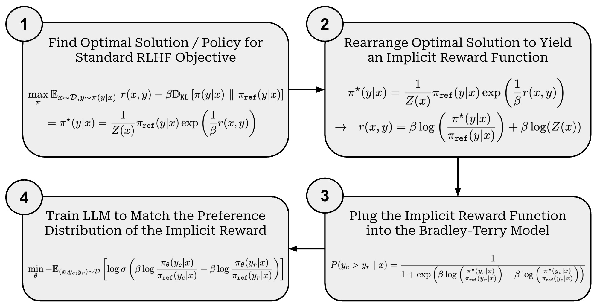
Proof sketch. Beginning with the standard RLHF training objective, we can derive the training loss used in DPO by following four key steps (shown above):
Deriving an expression for the optimal policy in RLHF.
Rearranging this expression to form an implicit reward function.
Putting the implicit reward into the Bradley-Terry preference model.
Training an LLM to match this implicit preference model—this is what we are doing in the DPO training process.
The above steps start with the objective used to train LLMs in RLHF and ends with the DPO loss function. In this derivation, we reformulate the RLHF optimization problem to arrive at the DPO training methodology. As we will see, RLHF and DPO are intricately related—they are trying to solve the same optimization problem! By studying the derivation below, we gain a deeper grasp of the relationship between these techniques.
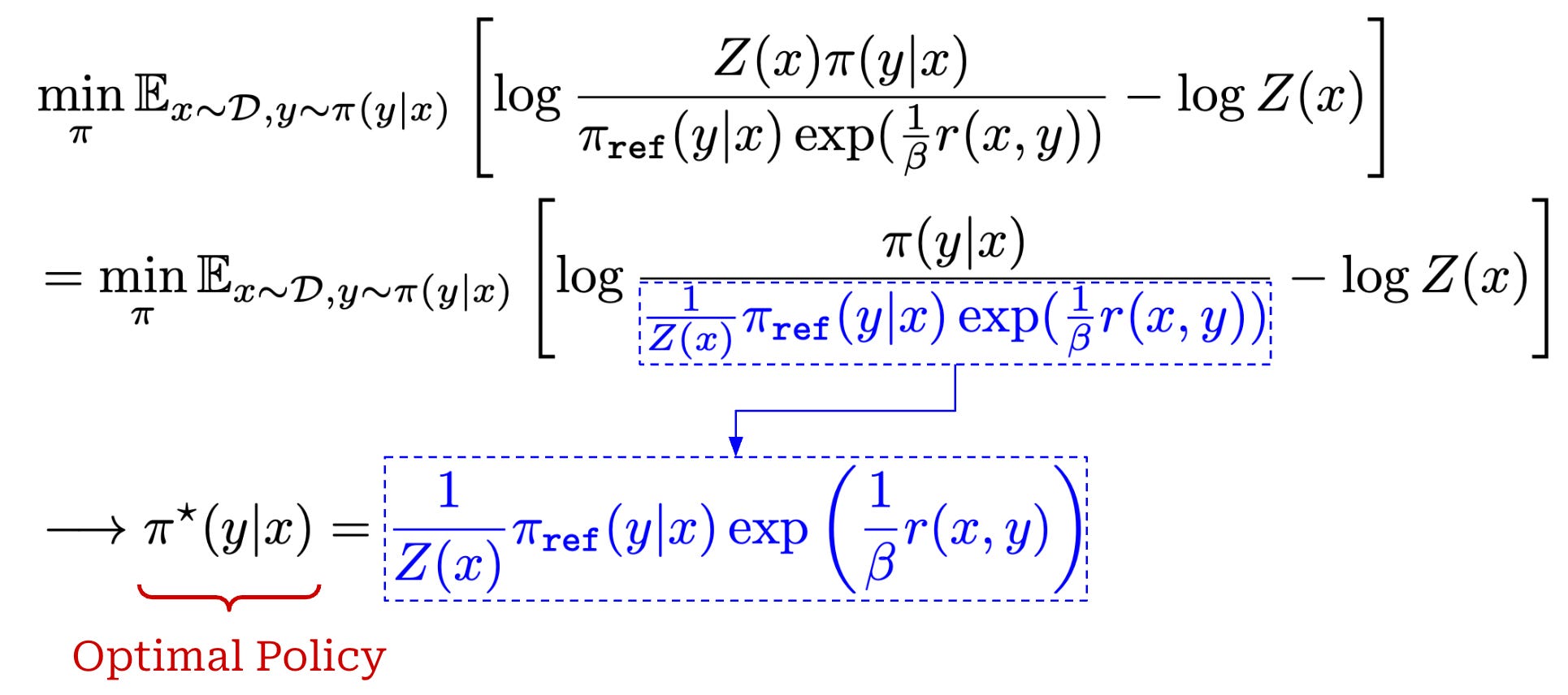
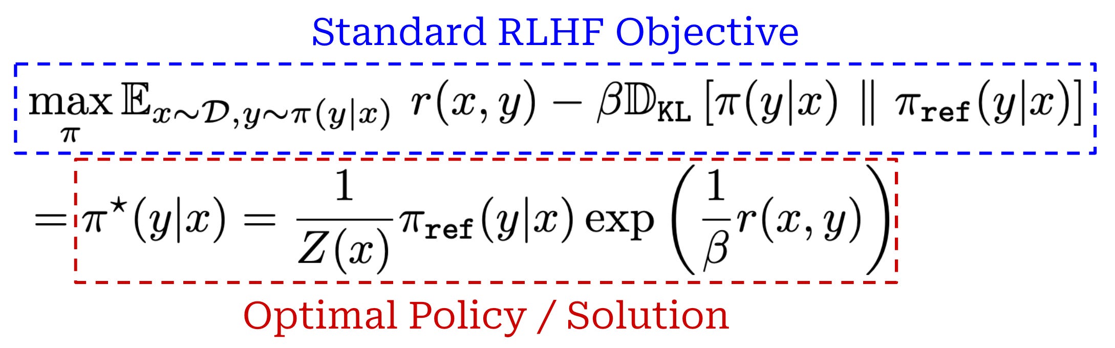
(Step One) Optimal solution to RLHF. To derive the DPO loss, we need to begin from the initial RLHF objective that we are trying to solve, which has been copied again below for readability. However, instead of using our learned reward model RM in this notation, we use a general reward function r(x, y). The general reward function can include—but is not limited to—our reward model.

Starting with this objective, we can follow the steps below to find a closed-form expression for the optimal solution to this objective. Put simply, we are solving for the value of π that actually maximizes the RLHF objective shown below!
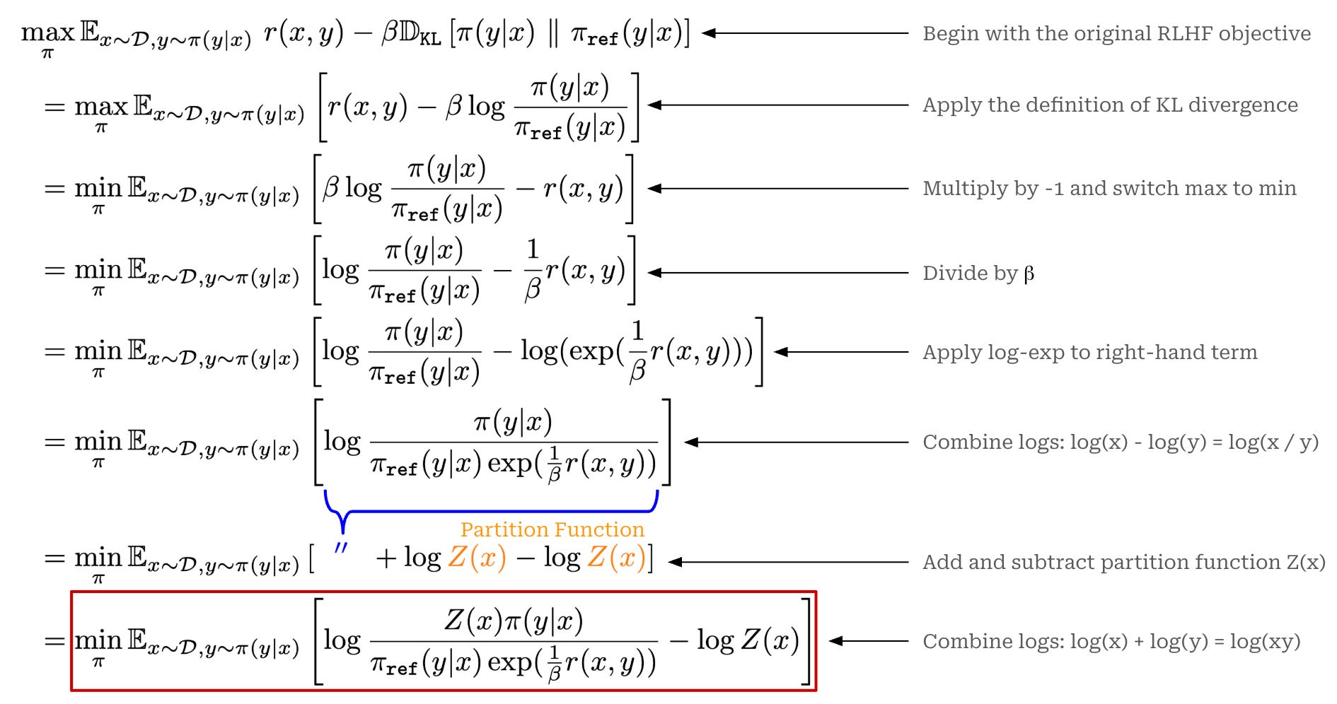
In the last two steps of the derivation above, we introduce a function Z(x), which we will call the partition function. The partition function is defined below. As we can see, the partition function only depends upon the reference policy and the input prompt x; there is no dependence upon the current policy or completion.

The name “partition function” is borrowed from fields like probability theory and statistical mechanics; see here. At the simplest level, the partition function is just a normalization term used in the theoretical derivation of DPO. We use Z(x) to ensure that the probability distribution we derive—in this case the optimal policy to the RLHF objective—sums to one and, therefore, forms a valid distribution.
Now that we understand the partition function, we will pick up the derivation from the equation in the red box shown above. Specifically, we will extract a portion of this term to define the expression below. We refer to this term as the “optimal policy”—the reason for this will become clear soon.
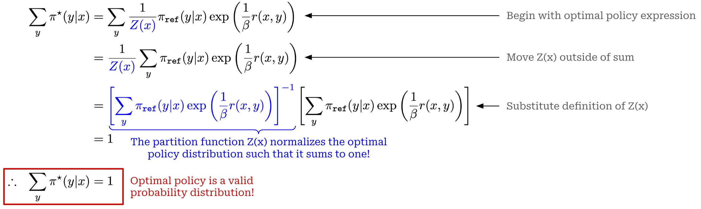
As mentioned before, the partition function is used as a normalization term for the optimal policy in the above expression. We know that the optimal policy defined above is a valid probability distribution because:
The value of the optimal policy is
≥0for all possible completionsy.The sum of the optimal policy across all completions
yis equal to1.
The first property is obvious—all components of the optimal policy are non-negative6. Proof of the second property is provided below, where we directly see how the partition function Z(x) is used to normalize the optimal policy distribution.
Now that we have defined (and verified the validity of) the optimal policy, we can return to the original expression in which this term appeared and substitute in the expression for the optimal policy. This yields the equation shown below.
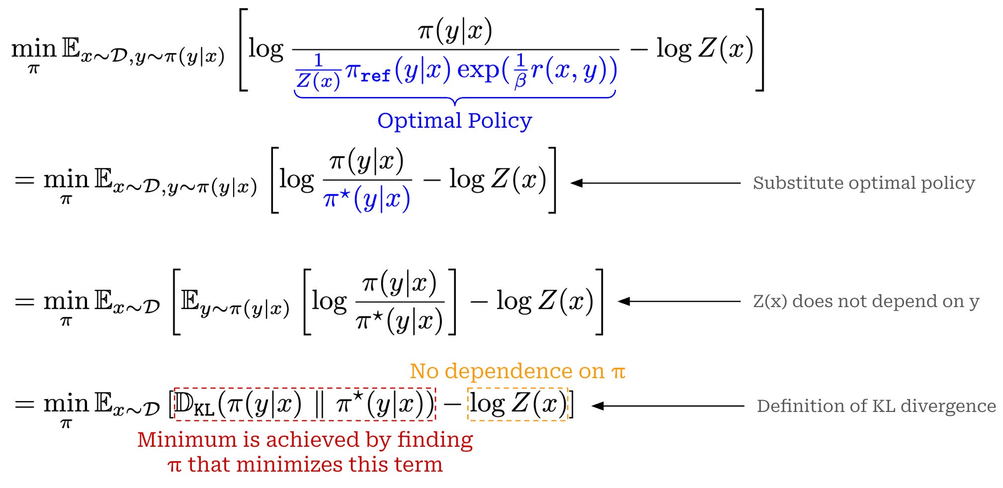
In the final term above, we see the crux of this derivation: the standard RLHF objective is minimized by finding the policy π that minimizes the KL divergence with the optimal policy. Since the KL divergence reaches its minimum value (zero) when the two probability distributions are identical7, the solution to this optimization is the optimal policy itself—hence the name. Therefore, we can express the optimal solution to the standard RLHF objective as shown in the equation below.
(Step Two) Deriving an implicit reward. From here, we can take our expression for the optimal policy shown above and rearrange it to derive an expression for the reward function—in terms of the optimal policy—as shown below.
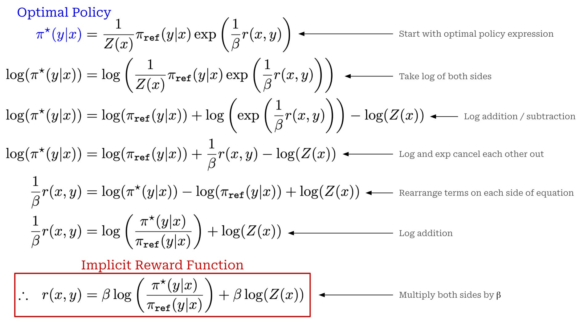
Now, we have derived a reparameterization of our reward. However, this reward function does not depend upon any explicit reward model. Rather, we estimate the reward purely using probabilities computed from the optimal policy and the reference policy—we will call this an “implicit” reward.
“This change-of-variables approach avoids fitting an explicit, standalone reward model… the policy network represents both the language model and the (implicit) reward.” - from [1]
Now, the only remaining issue is the Z(x) term in our implicit reward. The partition function takes a sum over all possible completions y, so computing the value of Z(x) is expensive in practice. Going further, the reward function r(x, y), which we cannot directly compute without training a standalone reward model, also appears in the expression for Z(x). To solve this, we need to revisit the Bradley-Terry model and combine it with our implicit reward function.
(Step Three) Bradley-Terry preference model. Under the Bradley-Terry model of preference, we can compute the probability that a given completion is preferred to another. In most cases, the input to this preference model is the explicit reward—predicted by a reward model—for each completion. In the case of DPO, we replace this explicit reward with our implicit reward function; see below.
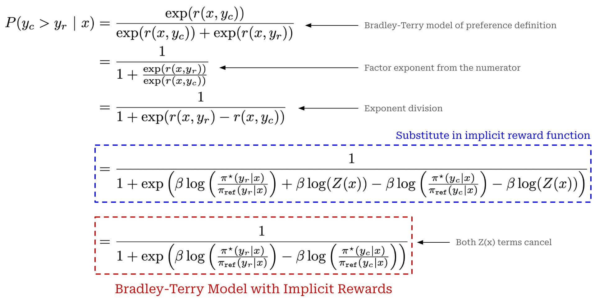
As shown in the final equation above, we now have an expression for the Bradley-Terry model of preference that uses our implicit reward function, where the implicit reward depends only upon the optimal policy and a reference policy. Due to the pairwise nature of the Bradley-Terry expression and the fact that the value of Z(x) depends only upon x (and not y), the Z(x) components of the implicit reward function actually cancel out when subtracting the implicit reward for the chosen completion from the implicit reward for the rejected completion.
(Step Four) Training our policy. The expression above depends upon the optimal policy, which is fixed—this optimal policy is the solution to the RLHF objective that we are trying to solve. From here, we must determine how to derive a training objective that can recover this optimal policy. To do this, DPO substitutes the optimal policy in the above expression with a learned policy, as shown below.
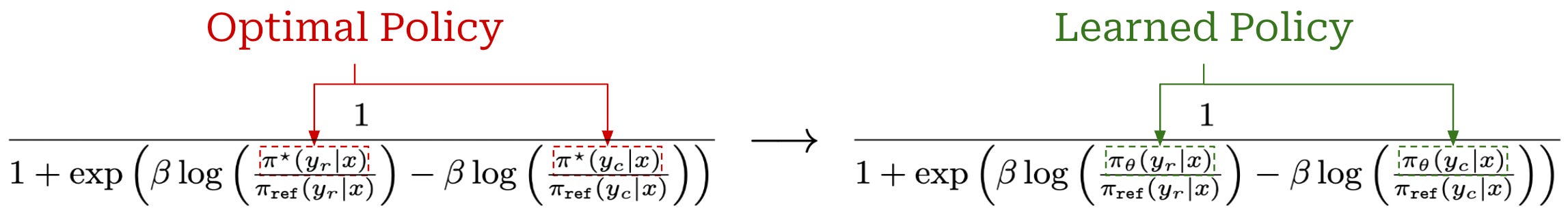
How can we make these two expressions equal? We need to train our learned policy! Specifically, we can formulate a ranking loss that optimizes our learned policy to empirically maximize the probability of chosen responses being preferred to rejected responses based on our implicit reward function. By doing this, we ensure that our preference model is accurate and, therefore, matches that of the optimal policy. Besides replacing explicit rewards with implicit rewards, this loss function is the same exact training objective used by standard reward models; see below.
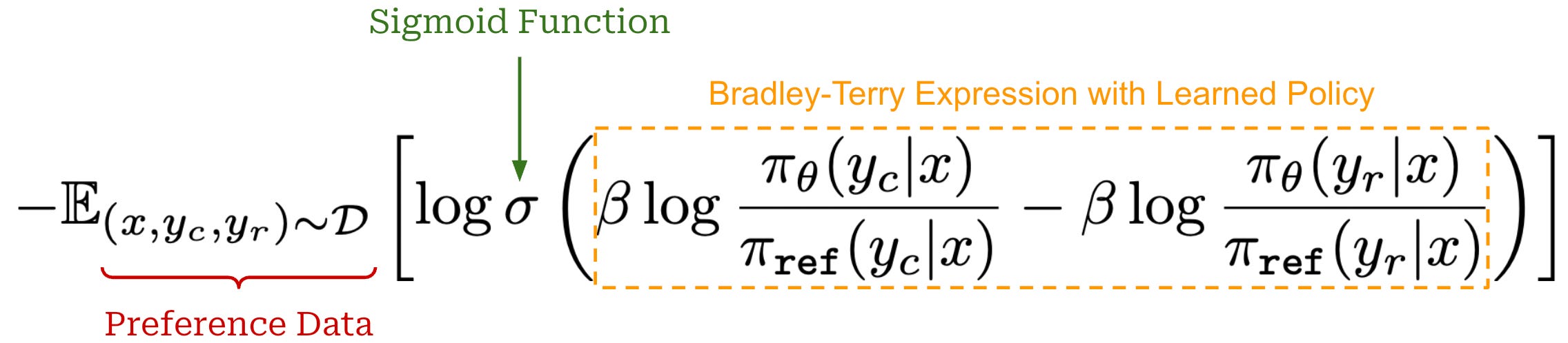
We might also notice that this loss function is identical to the training objective for DPO—we have now fully derived the DPO training objective starting from the training objective for RLHF. The training process for DPO learns an implicit reward model based upon our policy. By learning this implicit reward function, we obtain a policy that matches the optimal policy from RLHF.
Does DPO actually yield an optimal policy?
“The [DPO] optimization objective is equivalent to a Bradley-Terry model with an [implicit] reward parameterization and we optimize our parametric model equivalently to the reward model optimization… we show that [this objective] does not constrain the class of learned reward models and allows for the exact recovery of the optimal policy.” - from [1]
Based on the above derivation, training an LLM using the DPO loss will yield a model that has the same preference distribution—induced by the implicit reward—as the optimal policy. In other words, the implicit reward function learned by our policy via the DPO loss will correctly rank chosen and rejected completions in our preference dataset. However, the goal of DPO is not to train a model with a good implicit reward function—we want to align our LLM and derive a policy that generates high-quality completions! Luckily, authors in [1] provide a final proof showing that, in addition to learning a high-quality implicit reward function, the policy derived via DPO should match the optimal policy from RLHF.
Two reward functions r(x, y) and r’(x, y) are equivalent if and only if r(x, y) - r’(x, y) = f(x) for some function f(•).
Equivalent rewards. To begin the proof, we can first specify an equivalence relation for reward functions. This is just a definition that captures what it means for two reward functions to be equal; see above. Put simply, reward functions are considered equivalent if their difference in reward only depends upon the prompt and not the completion. Using this definition, we show below that two equivalent reward functions are guaranteed to yield the same preference distribution8.
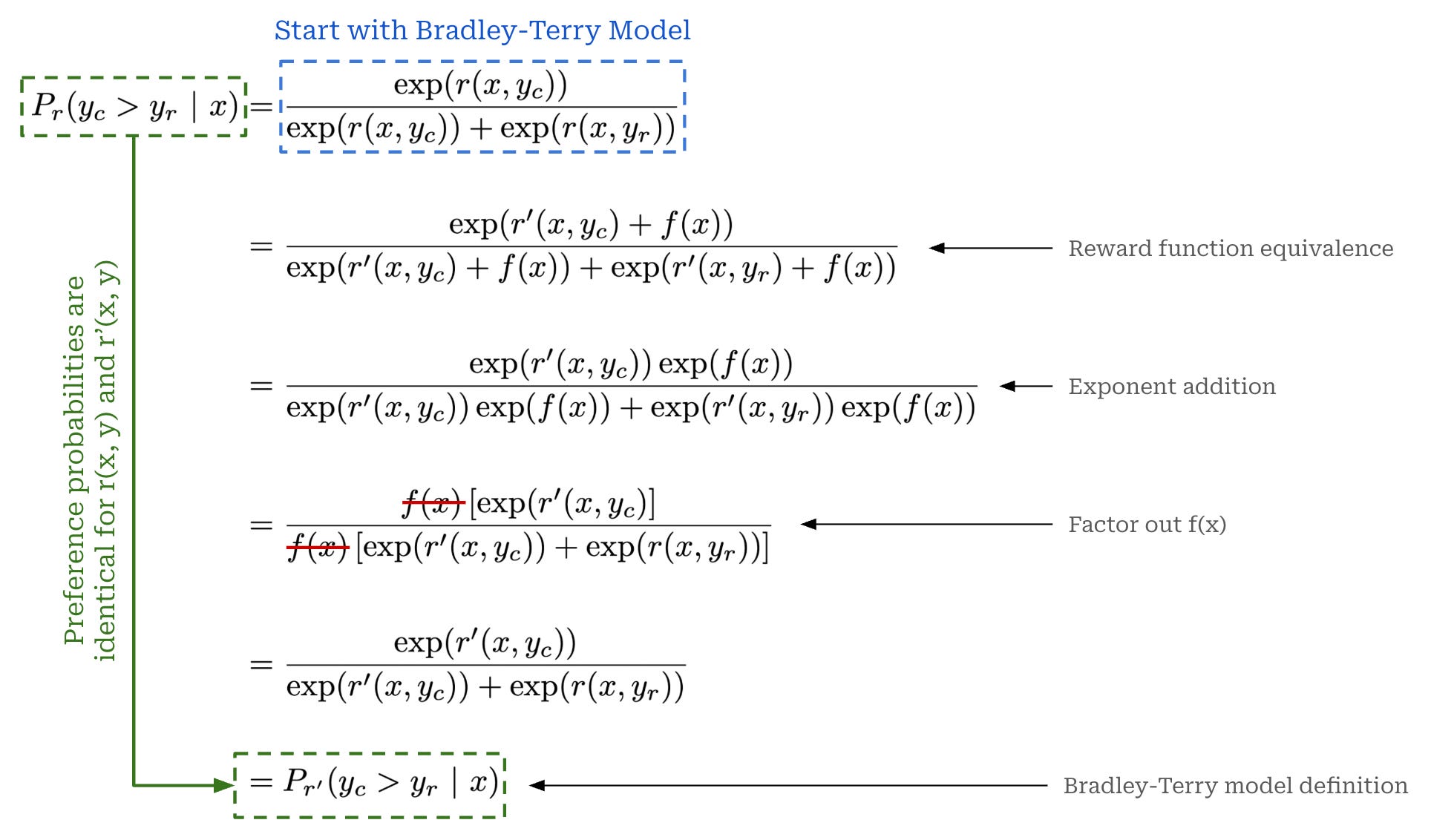
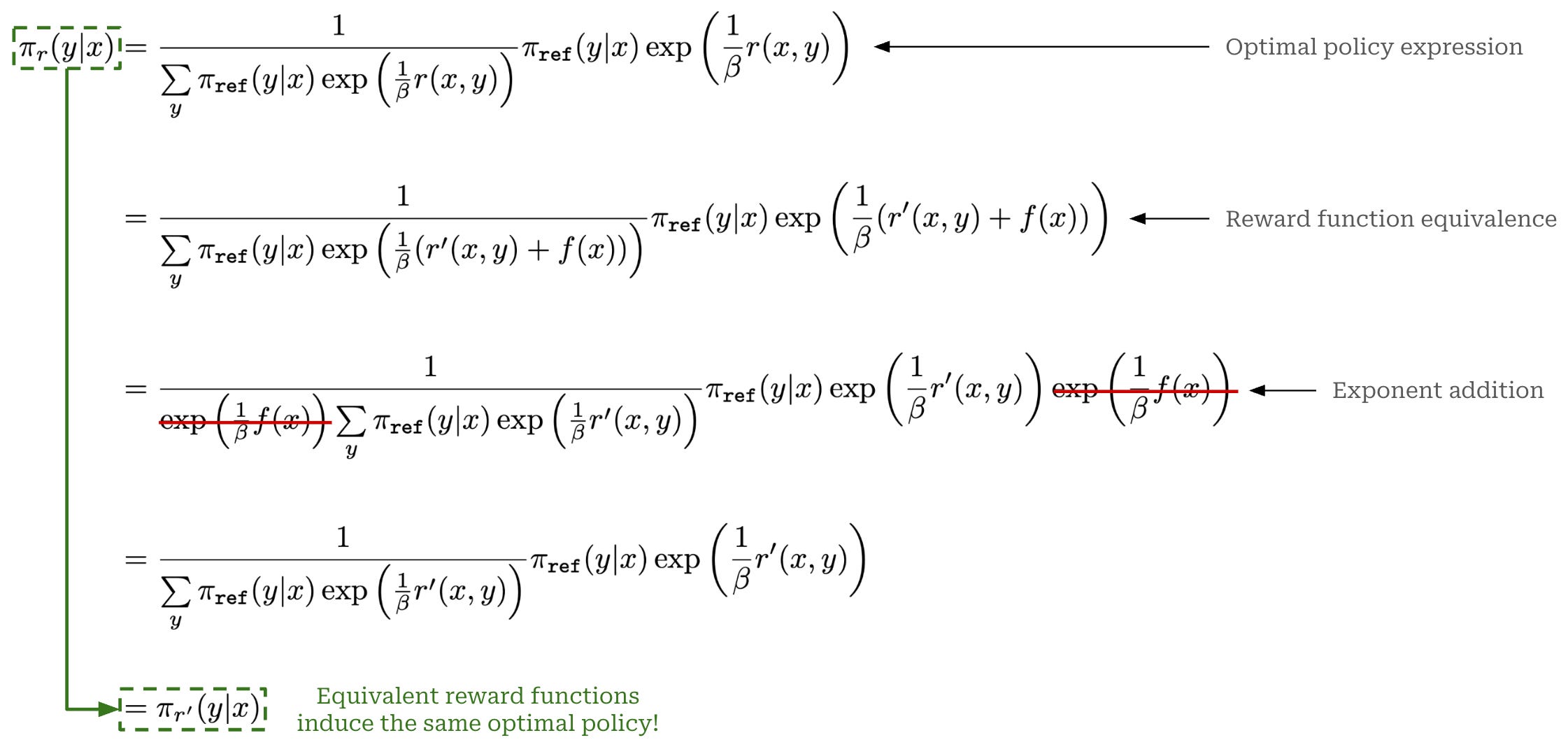
We can also write a similar proof to show that two equivalent reward functions, when plugged into the standard RLHF objective that we explored in the prior section, are guaranteed to yield the same optimal policy; see below.
Proving an optimal policy. Given the above results, the last step in this proof is to simply show that the implicit reward function used within DPO is equivalent to the actual reward used within RLHF. If these two reward functions satisfy the equivalence relation, then we know that DPO will yield the same optimal policy as RLHF based on the findings shown above. To prove this final result, we can start by considering an arbitrary reward function r(x, y) used by RLHF. Our goal is to show that the implicit reward from DPO is equivalent to r(x, y).
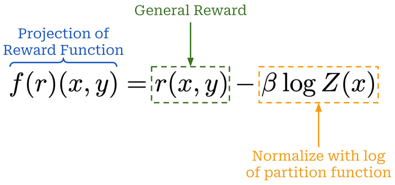
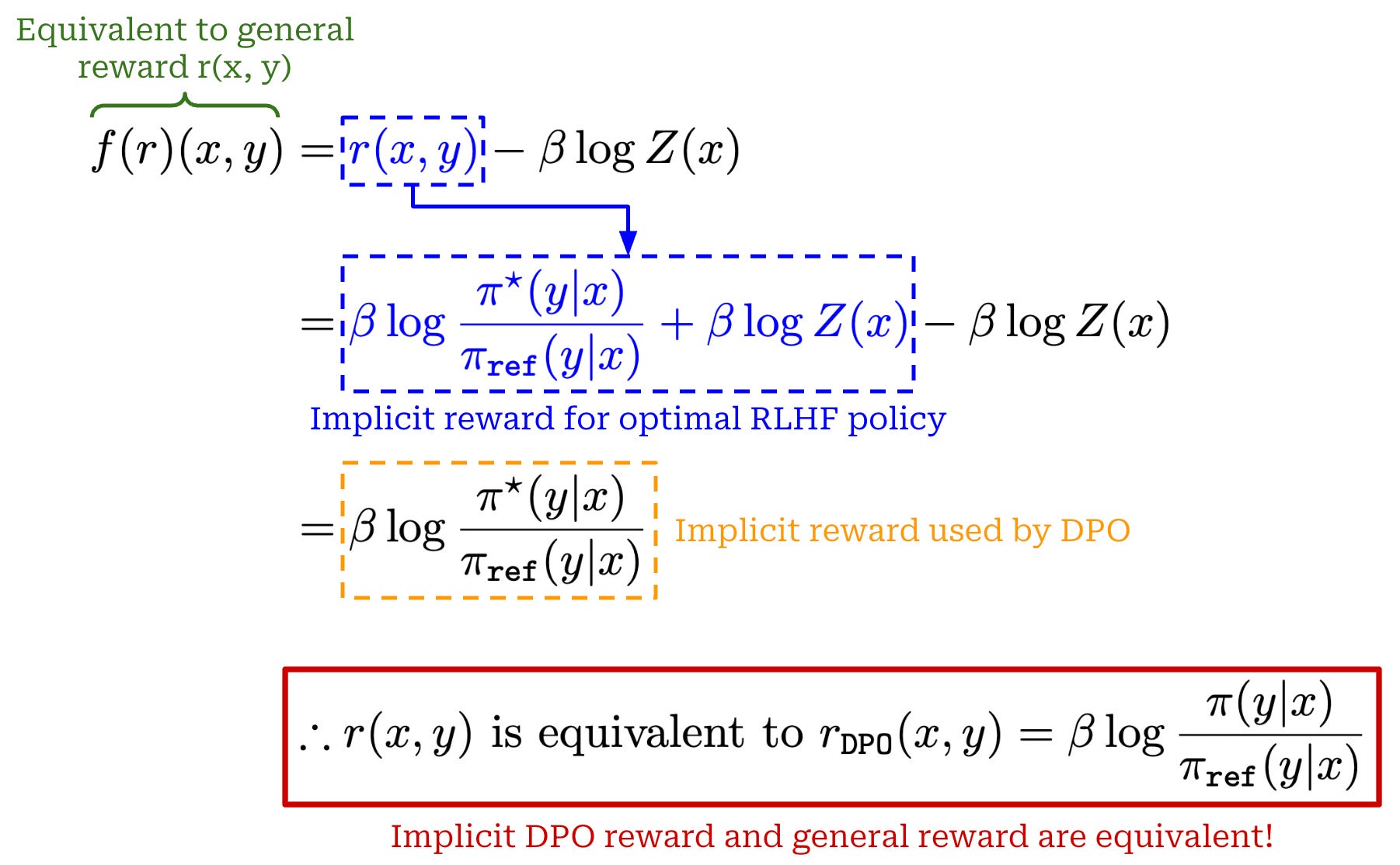
Given an arbitrary reward, we can define the modified9 reward expression shown above. This expression just subtracts an extra term (i.e., the log of the partition function) from r(x, y). Notice also that the term we subtract from r(x, y) only depends on x. For this reason, the modified reward expression is equivalent to r(x, y) according to the equivalence relation that we defined earlier.
“The second lemma states that all reward functions from the same class yield the same optimal policy, hence for our final objective, we are only interested in recovering an arbitrary reward function from the optimal class.” - from [1]
To prove the desired result, we have to draw upon our prior expression that rearranges the optimal RLHF solution to produce an implicit reward. If we plug this implicit reward into the modified reward expression above, we get a reward—which is known to be equivalent to r(x, y)!—that matches the implicit reward in DPO; see below. As a result, we now know that the implicit reward used by DPO satisfies the equivalence relation with r(x,y), which completes the proof.
Key takeaway. Before we conclude this section, we should quickly contextualize the result that we just proved. In the prior section, we derived an expression for the preference distribution induced by the implicit reward of the optimal policy (or solution) to the standard RLHF objective. After this expression is derived, we can easily train a model to have an implicit reward function that matches this preference distribution by adopting the same training strategy as a normal reward model. Therefore, the key training procedure behind DPO centers around training an (implicit) reward model, hence the name of the paper; see below.
A common misconception of DPO is that it removes the reward model, which is not true. In fact, DPO is completely based upon reward modeling. The reward model is just implicit, which means we can avoid training an explicit reward model.
“What is often misunderstood is that DPO is learning a reward model at its core, hence the subtitle of the paper Your Language Model is Secretly a Reward Model. It is easy to confuse this with the DPO objective training a policy directly” - RLHF book
Given that the training procedure for DPO is based upon reward modeling, it’s not immediately obvious that training an LLM in this way will actually yield an optimal policy. Could our resulting model have an accurate implicit reward function but still not generate high-quality completions? In this section, we prove this should not be the case. If we train a model to match the implicit preference distribution of the optimal policy, then the resulting policy is also guaranteed to be optimal! Put simply, DPO indirectly provides us with a policy that is comparable in quality to one derived via training with RLHF, making it a valid preference tuning alternative that is significantly less complex than techniques like PPO-based RLHF.
Why does DPO work?
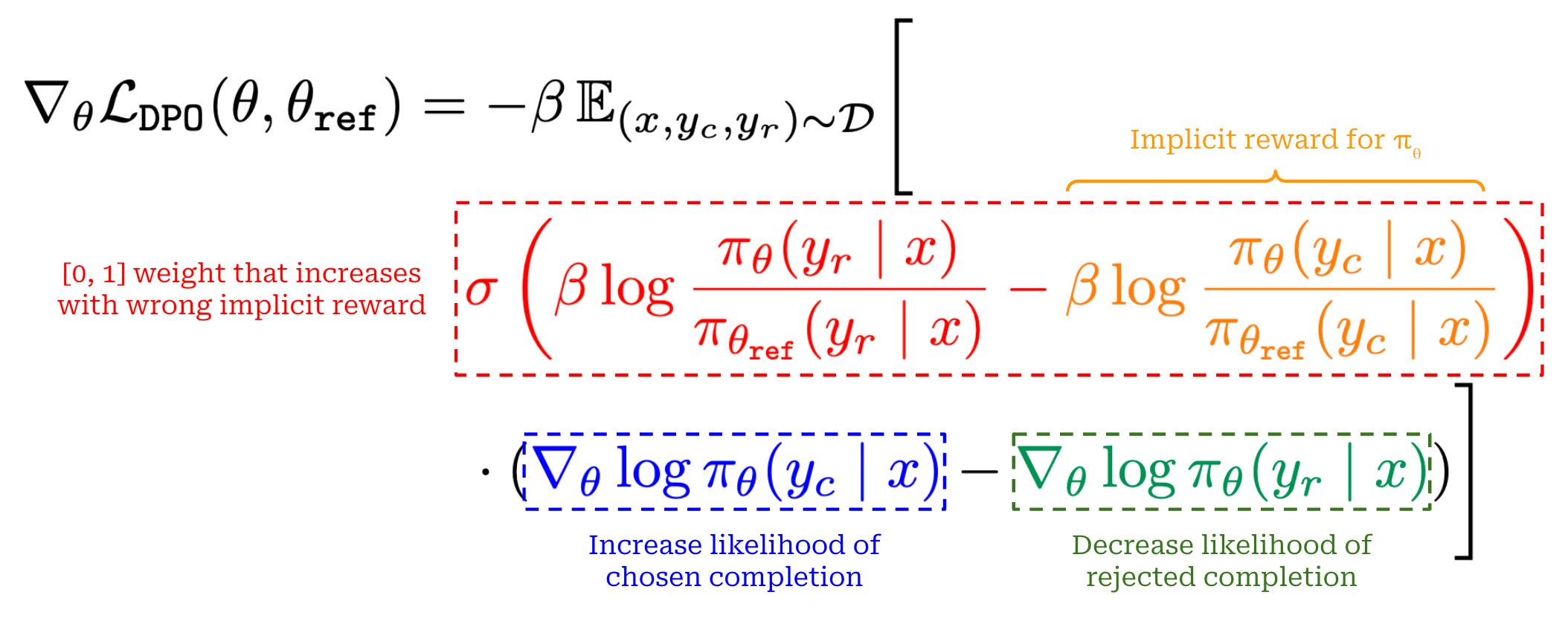
To gain a deeper understanding of DPO and why it works well, we can look at the structure of the gradient for DPO’s loss function; see above10. There are three key terms in this expression, colored in red (with part of the term in orange), blue and green for clarity. The purpose for each of these terms is as follows:
The first (red) term is a weight—falling in the range
[0, 1]due to the sigmoid function—that increases as the implicit reward of the rejected completion increases relative to that of the chosen completion. In other words, this term assigns a higher weight to implicit reward estimates that are wrong.The second (blue) term is the positive gradient of the likelihood for the chosen completion with respect to the LLM’s parameters, which serves the purpose of increasing the likelihood for the chosen completion.
The third (green) term is the negative gradient of the likelihood for the rejected completion with respect to the LLM’s parameters, which serves the purpose of decreasing the likelihood for the rejected completion.
These terms work together to simultaneously i) increase the likelihood of chosen completions and ii) decrease the likelihood of rejected completions, where extra emphasis (i.e., a larger update to our LLM’s parameters) is placed upon cases where the implicit reward estimate assigned by our LLM is incorrect.
“Examples are weighed by how much higher the implicit reward model rates the dispreferred completions scaled by beta… how incorrectly the implicit reward model orders the completions, accounting for the strength of the KL constraint.” - from [1]
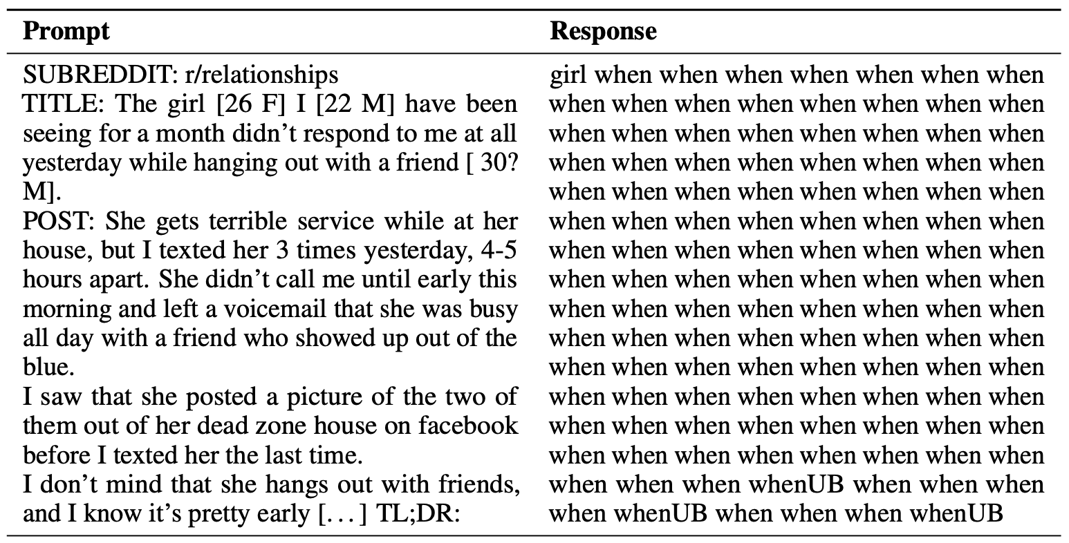
Weighting coefficient. Authors in [1] observe that all three sub-components of DPO’s loss gradient are necessary for the algorithm to work well. Notably, if we remove the first weighting term from this gradient—creating a gradient that uniformly increases the likelihood of all chosen completions and decreases the likelihood of all rejected completions—the resulting policy is low-quality and even tends to completely degenerate when generating text; see below. Such a training algorithm is called unlikelihood training and has been explored in the past [5]. The simple weighting term added to the loss gradient by DPO completely transforms this approach, making it capable of performing high-quality LLM alignment.
Implementing DPO from Scratch
Although the derivation of DPO is complex, the technique is actually quite simple to use practically. In fact, DPO played a huge role in democratizing research on LLM post-training for those outside of top labs [3]. Algorithms like PPO-based RLHF are harder to tune and require significant compute resources. In contrast, DPO uses a standard classification (or ranking) loss with no RL and only keeps two copies of the model—instead of four—throughout the training process.
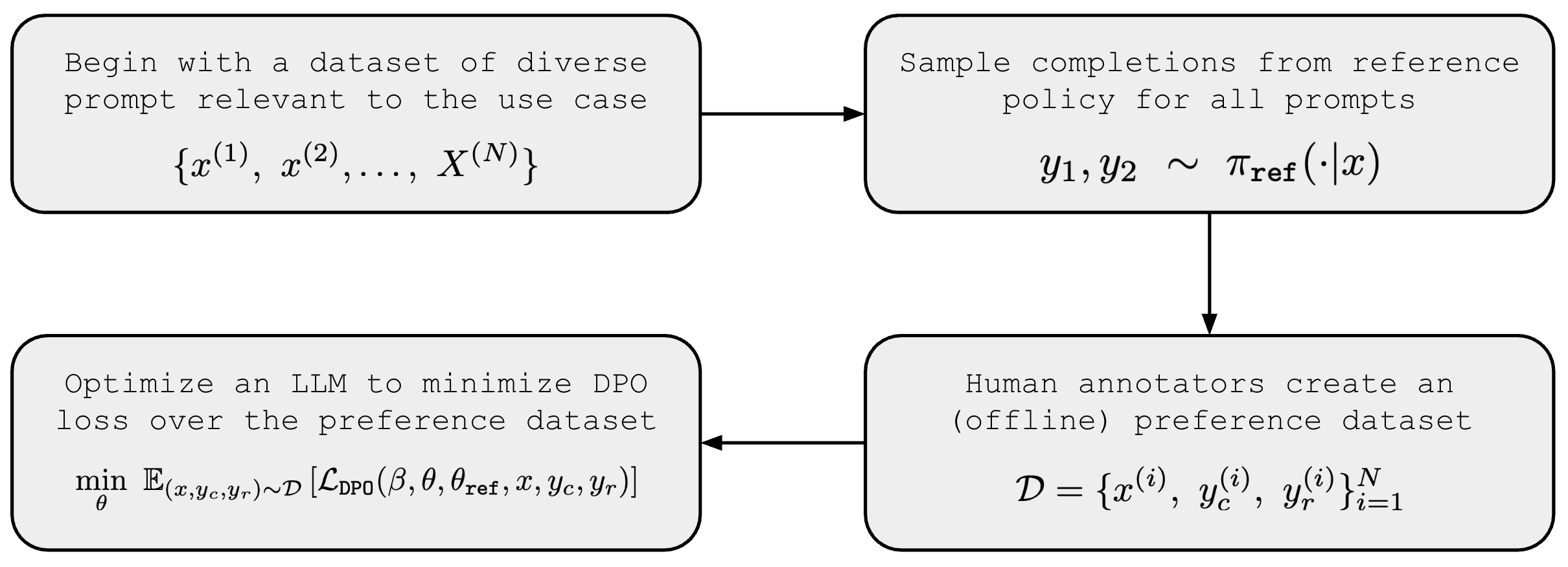
DPO training pipeline. The standard training process with DPO is depicted above. We begin the process with a diverse set of prompts that capture the use case(s) for which we are training our model. From here, we use our reference policy to generate pairs of completions for each prompt and have human raters provide preference annotations for each pair. Once this preference dataset is available, we perform maximum likelihood estimation by training our model to minimize the DPO loss that we derived earlier over the preference dataset.
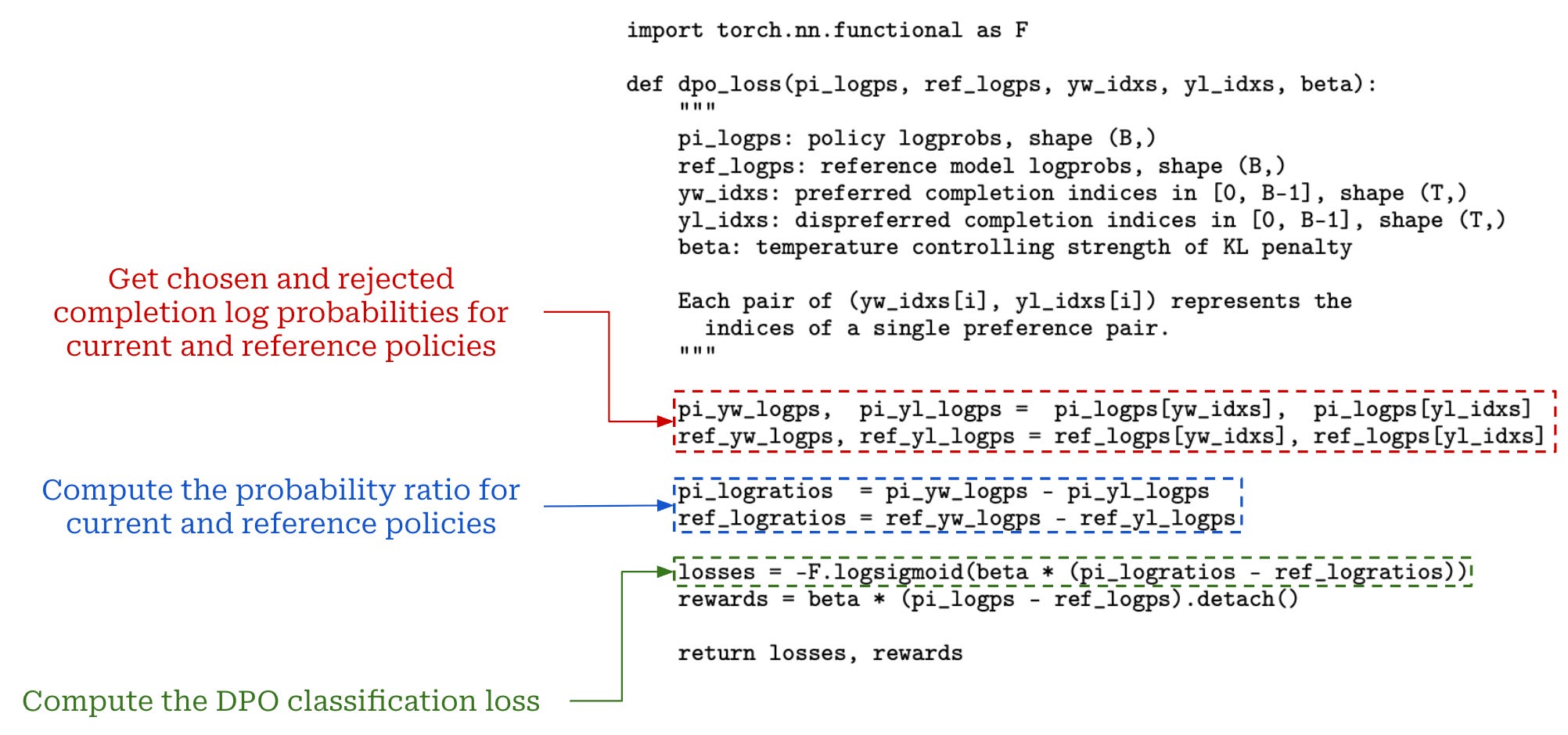
Loss implementation. We can pretty easily implement the loss function for DPO in PyTorch—it is just a ranking loss applied over implicit rewards derived from the current and reference policies. The example implementation of the loss from [1] is copied below for reference, where we see that the loss is computed by:
Getting the log probabilities assigned to each completion—both chosen and rejected—by the current policy and the reference policy.
Computing the probability ratio between chosen and rejected completions for both the current policy and the reference policy.
Using the above probability ratios to construct the final DPO loss.
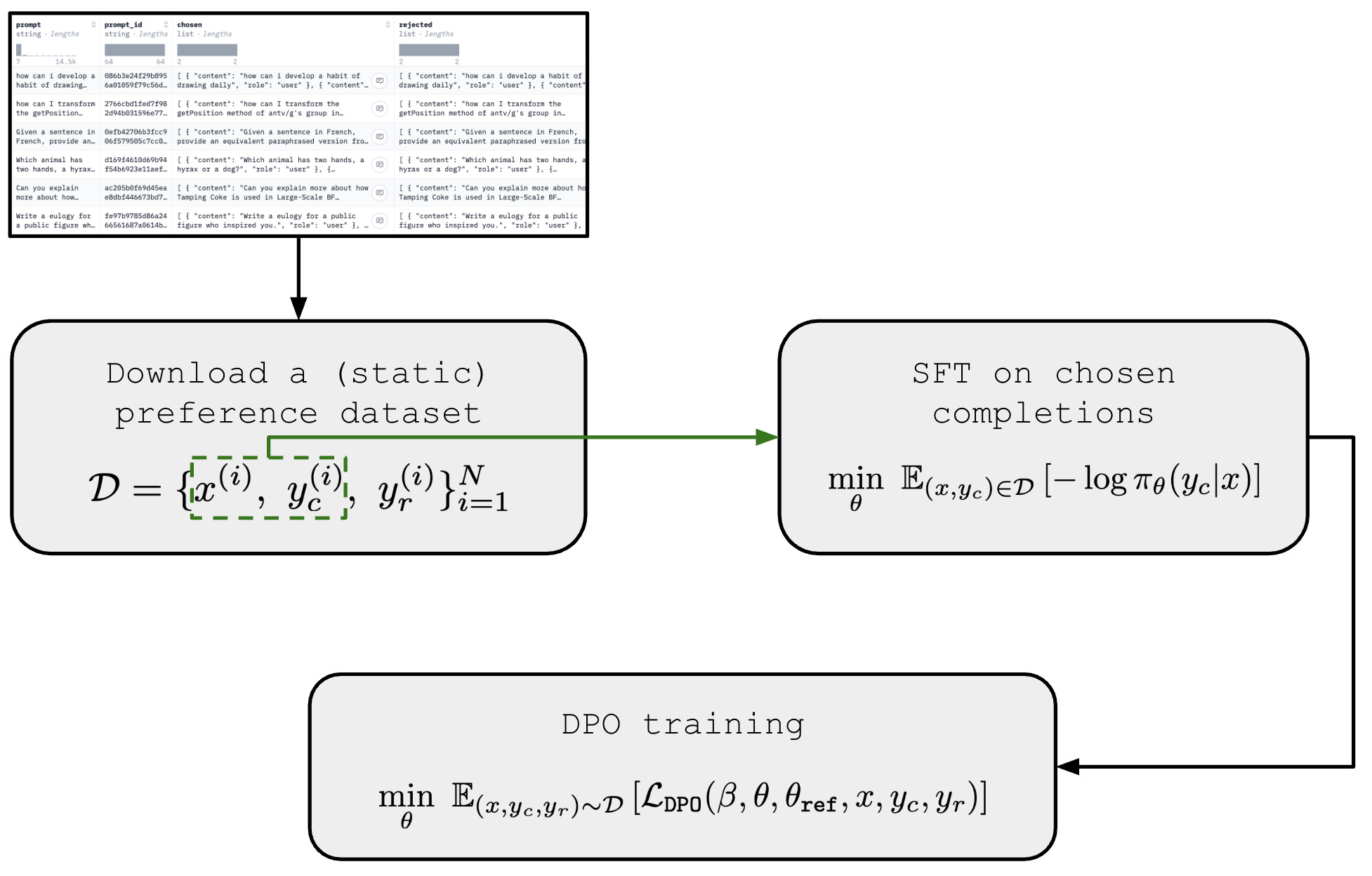
Handling offline preference data. DPO is fundamentally an offline preference learning algorithm—we are optimizing our model over a static preference dataset. In the pipeline outlined above, we use our reference model to generate completions in our preference dataset. In most practical applications, however, this may not be the case. As a practitioner, we may simply download a preference dataset like UltraFeedback [4] online and train our model over this static dataset using DPO. In such cases, the actual reference model is unknown and may be different from the reference model we used in DPO training, creating a distribution shift.
“Since the preference datasets are sampled using the SFT model, we initialize the reference policy to the SFT model whenever available. However, when the SFT model is not available, we initialize the reference policy by maximizing likelihood of preferred completions. This procedure helps mitigate the distribution shift between the true reference distribution and the reference policy used by DPO.” - from [1]
To minimize this distribution shift and ensure that the actual reference model aligns well with the completions present in our preference dataset, authors in [1] recommend the procedure depicted below. In this procedure, we first perform supervised finetuning of our reference model on the chosen completions in the preference dataset, then further train this model with DPO afterwards. This preliminary SFT training stage ensures the reference policy in DPO is not too different from the true reference policy used to create the preference dataset.
The last consideration for implementing DPO is correctly setting the β hyperparameter, which controls the amount that the trained policy can differ from the reference policy. Remember, β is the weight by which we multiply the KL constraint in the RLHF objective, which controls the strength of preference alignment in DPO—lower β values mean that the model is updated more aggressively to adapt to observed preference in the data. Usually, β is set to a value in the range [0, 1], where lower values are more common. For example, β = 0.1 is a popular choice, though authors in [1] explore both β = 0.1 and β = 0.5.
Full DPO example. One of the easiest ways to finetune your own LLM with DPO is by using the DPOTrainer in the HuggingFace TRL package. To perform a DPO training run, you just need to i) load a preference dataset like UltraFeedback; ii) choose a model / tokenizer (e.g., a smaller model like Qwen3-0.6B is great if we don’t have big GPUs); and iii) execute the DPO trainer as shown in the code below.
from trl import DPOConfig, DPOTrainer

# load model and data
model = <load our model>
tokenizer = <load our tokenizer>
train_dataset = <load our preference dataset>

# configure DPO training process training_args = DPOConfig(output_dir="./dpo_logs/")
trainer = DPOTrainer(
    model=model,
    args=training_args,
    processing_class=tokenizer,
    train_dataset=train_dataset,
)

# execute DPO training
# run the below command to execute this script
# > accelerate launch <script name>
trainer.train()
Summary and Key Takeaways
Direct Preference Optimization (DPO) is a preference-tuning method for LLMs that indirectly solves the RLHF objective while avoiding explicit reward models and RL. In DPO, we reparameterize the RLHF objective to form an implicit reward function derived from the policy itself (and a reference policy). Then, we train our LLM over a static preference dataset to optimize this implicit reward function, similarly to a standard reward model. By solving this implicit reward modeling objective, we indirectly yield a policy that solves the RLHF objective.
This approach offers a simpler, more stable, and computationally efficient alternative to RL-based alignment methods, making high-quality LLM alignment more accessible. However, several works have studied the differences between (offline) direct alignment algorithms like DPO and alignment techniques that use online RL (e.g., PPO-based RLHF), finding that a performance gap can exist [11, 12]. Despite this fact, DPO is still heavily used in LLM post-training—often in tandem with online algorithms—due to its simplicity and effectiveness.
New to the newsletter?
Hi! I’m Cameron R. Wolfe, Deep Learning Ph.D. and Senior Research Scientist at Netflix. This is the Deep (Learning) Focus newsletter, where I help readers better understand important topics in AI research. The newsletter will always be free and open to read. If you like the newsletter, please subscribe, consider a paid subscription, share it, or follow me on X and LinkedIn!
Bibliography
[1] Rafailov, Rafael, et al. "Direct preference optimization: Your language model is secretly a reward model." Advances in neural information processing systems 36 (2023): 53728-53741.
[2] Stiennon, Nisan, et al. "Learning to summarize with human feedback." Advances in neural information processing systems 33 (2020): 3008-3021.
[3] Tunstall, Lewis, et al. "Zephyr: Direct distillation of lm alignment." arXiv preprint arXiv:2310.16944 (2023).
[4] Cui, Ganqu, et al. "Ultrafeedback: Boosting language models with scaled ai feedback, 2024." URL https://arxiv. org/abs/2310.01377.
[5] Welleck, Sean, et al. "Neural text generation with unlikelihood training." arXiv preprint arXiv:1908.04319 (2019).
[6] Lambert, Nathan, et al. "Tulu 3: Pushing frontiers in open language model post-training, 2024." URL https://arxiv. org/abs/2411.15124 297 (2025).
[7] Yang, An, et al. "Qwen3 technical report." arXiv preprint arXiv:2505.09388 (2025).
[8] Dubey, Abhimanyu, et al. "The llama 3 herd of models." arXiv e-prints (2024): arXiv-2407.
[9] Kaplan, Jared, et al. "Scaling laws for neural language models." arXiv preprint arXiv:2001.08361 (2020).
[10] Sheng, Guangming, et al. "Hybridflow: A flexible and efficient rlhf framework." Proceedings of the Twentieth European Conference on Computer Systems. 2025.
[11] Tang, Yunhao, et al. "Understanding the performance gap between online and offline alignment algorithms." arXiv preprint arXiv:2405.08448 (2024).
[12] Ivison, Hamish, et al. "Unpacking dpo and ppo: Disentangling best practices for learning from preference feedback." Advances in neural information processing systems 37 (2024): 36602-36633.
More specifically, "online" means that the policy is updated iteratively with new samples generated at each step, while "offline" means that all training data is fixed in advance.
The word “policy” is RL jargon for the LLM or model that we are training (with RL).
More specifically, the KL divergence is measuring how much information is lost when the given distribution is used to approximate the reference distribution.
The reference model is not always the SFT model. It can also be a previous model checkpoint from RL training. For example, if four phases or rounds of RLHF are performed sequentially, then the reference model for the second phase of RLHF could be the model resulting from the first phase of RLHF.
The optimal policy is a product of the partition function, the reference policy, and an exponential function, all of which cannot be less than zero. Therefore, the product of these terms, which form the optimal policy, must also be non-negative.
This is known due to Gibbs’ inequality.
In [1], this proof is provided assuming the more general Plackett-Luce model (see Appendix A.5 on page 17), but we rewrite this proof using the Bradley-Terry model for simplicity and to match the rest of the explanation in this overview.
In [1], authors describe this modified function as a “projection” of the reward function.
Remember, DPO trains the LLM using MLE. In other words, our LLM’s parameters are directly updated by repeatedly i) computing this gradient over a batch of data, ii) multiplying the gradient by a scalar factor (i.e., the learning rate), and iii) subtracting this scaled gradient from our model parameters. If you want to understand how this gradient is derived, please see page 17 of this paper.
gosh, DPO is so forgotten man, was such a major innovation.
You have become my fav!