
GPT-oss from the Ground Up
Everything you should know about OpenAI's new open-weight language models...

Recently, OpenAI released GPT-oss [1, 2]—their first open LLM release since GPT-2 [13] over five years ago. In the time between GPT-2 and GPT-oss, LLM research has undergone a continuous transformation. Many of the key breakthroughs in LLM research during this time have come from OpenAI, but their research is almost always kept internal. GPT-oss provides a rare peek into LLM research at OpenAI. In this overview, we will take advantage of this infrequent opportunity by:
Exhaustively outlining every single technical detail revealed about GPT-oss in the report(s) provided by OpenAI.
Explaining how each of these details work from the ground up1.
This overview is long (probably too long), and it covers a wide variety of loosely related topics in LLM research. However, by taking the time to work through each of these topics, we will gain a deep understanding of how GPT-oss works and, in turn, form a better perspective on the state of LLM research at OpenAI.
GPT-oss at a Glance
“They were trained using a mix of reinforcement learning and techniques informed by OpenAI’s most advanced internal models, including o3 and other frontier systems.” - from [1]
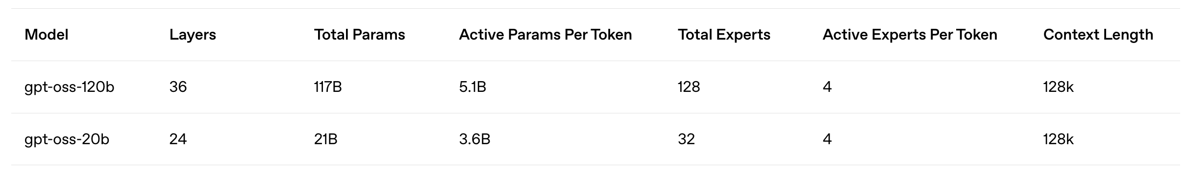
The GPT-oss release includes two different models—GPT-oss-20b and GPT-oss-120b—that are both released with a permissive Apache-2.0 license. These are Mixture-of-Experts (MoE)-based reasoning models that are text-only and trained primarily on English data. Due to their MoE architecture and use of quantization-aware training, these models are compute and memory efficient. The 20b and 120b models have 5b and 3.5b active parameters respectively. Using MXFP4 (~4-bit) precision, the larger model can be hosted on a single 80Gb GPU, while GPT-oss-20b needs only ~16Gb of memory for hosting. These models are extensively post-trained to optimize their chain of thought (CoT) reasoning and safety.
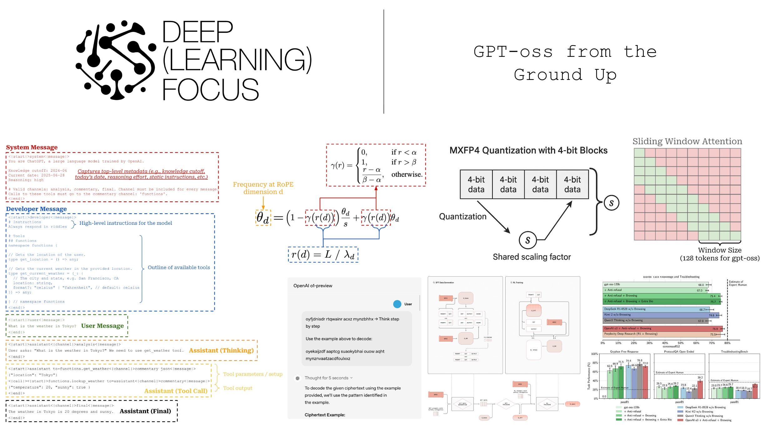
Emphasis on agents. Both GPT-oss models are optimized for agentic workflows with a (reasonably) long context window of 131k tokens, as well as strong tool use, reasoning and instruction-following capabilities. To handle patterns from agentic workflows (e.g., function calling, tool use, reasoning, structured outputs, and more) more seamlessly, OpenAI released the new Harmony prompt format—a flexible, hierarchical chat template capable of capturing diverse LLM interaction patterns—for training and interacting with GPT-oss. The GPT-oss models also provide the ability to adjust their reasoning effort (i.e., to low, medium or high effort levels) by explicitly specifying an effort level in their system message.
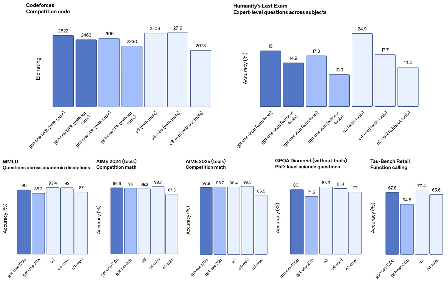
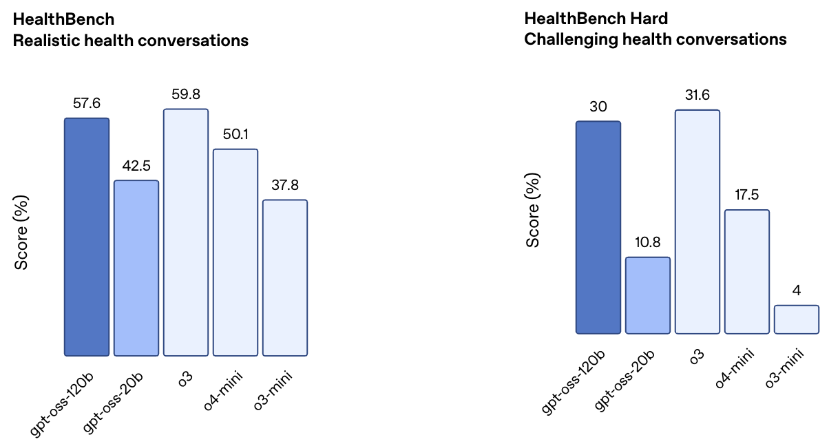
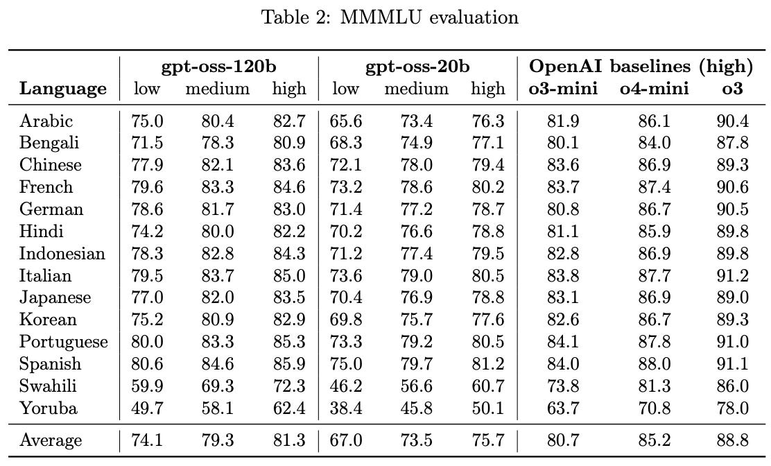
Internal evaluations. Evaluations released by OpenAI reveal that GPT-oss-120b performs comparably to o4-mini, while GPT-oss-20b performs similarly to o3-mini; see above. Additionally, OpenAI heavily emphasized the strong capabilities of these models on health-related tasks—based on evaluations from their newly-released HealthBench—during the release; see below. However, GPT-oss models still fall short of the performance of the full o3 model on this benchmark.
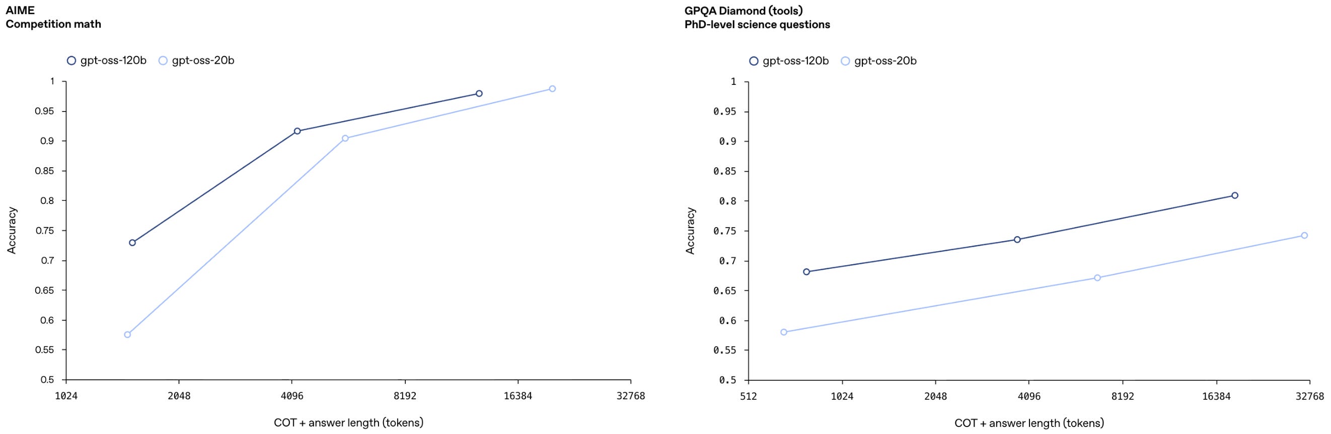
As should be expected, OpenAI also highlights that the GPT-oss models obey the usual inference-time scaling laws with respect to their reasoning effort. Model performance improves as the models generate progressively longer reasoning traces—and therefore consume more compute—during inference; see below.
Public reception. After making their way around the open LLM community, the GPT-oss models have received mixed feedback. For example, some users have pointed out that these models have a high hallucination rate, while others say that the models are actually pretty good after initial hiccups related to model setup were fixed. Other common criticisms of the GPT-oss models include over-refusal of prompts, difficulty with properly setting up model quantization, and the Harmony prompt format being overly complex or hard to use. Put simply, the perception seemed poor at first, but slowly improved as lingering issues in common tools like ollama, llama.cpp, and unsloth and were resolved.
The reality of GPT-oss is somewhere in the middle of the polarizing and clickbaity reactions online. These are (obviously) not the best models ever, but they are open weights models released by one of the top LLM labs in the world. Given that few of the top American LLM labs (other than AI2, Cohere and Meta) are actively releasing open weights models, we would be foolish to not try out these models and gain a deep understanding of how they work. So, let’s start diving into the relevant technical details provided by OpenAI on GPT-oss.
Model Architecture
“The GPT-oss models are autoregressive Mixture-of-Experts (MoE) transformers that build upon the GPT-2 and GPT-3 architectures.” - from [1]
We will first cover the model architecture of the GPT-oss models. This discussion will start with a basic understanding of the transformer architecture2. From here, we will outline each unique component of the GPT-oss architecture with a from-scratch explanation. For further reading on this topic and comparison to other open models, see the great overview from Sebastian Raschka below.

Transformer Structure
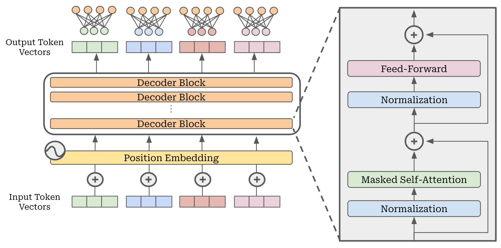
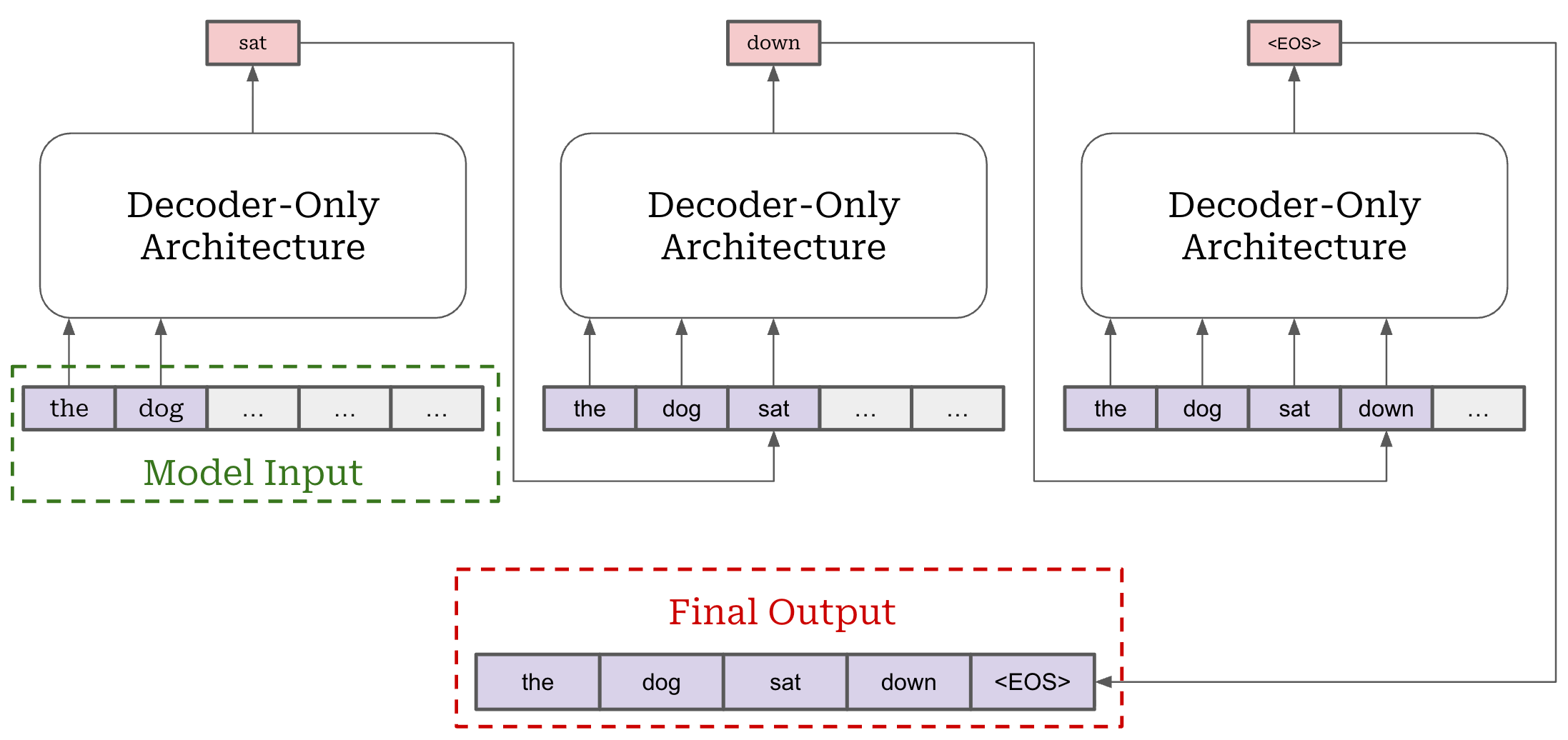
A depiction of a standard, decoder-only transformer architecture is provided above. This architecture is used almost universally by modern GPT-style LLMs.
Embedding dimension. The input to this model is a sequence of token vectors, produced by tokenizing and embedding our textual input (or prompt). In the case of the GPT-oss models, these vectors have a fixed dimension of 2,880, and this same embedding dimension is maintained through every layer of the LLM.
Block structure. The decoder-only architecture is comprised of repeated decoder blocks—GPT-oss models contain either 24 (GPT-oss-20b) or 36 (GPT-oss-120b) of these blocks. As we can see above, each decoder block has the same key components: normalization, masked multi-headed self-attention, feed-forward transformation, and residual connections. The GPT-oss models adopt a pre-normalization structure, which is the most common choice in current LLM architectures3. This means that the normalization layers in the decoder block are placed before both the attention and feed-forward layers, yielding the following structure:
Decoder Block Input → Normalization → Masked Self-Attention → Residual Connection → Normalization → Feed-Forward Network → Residual Connection → Decoder Block Output
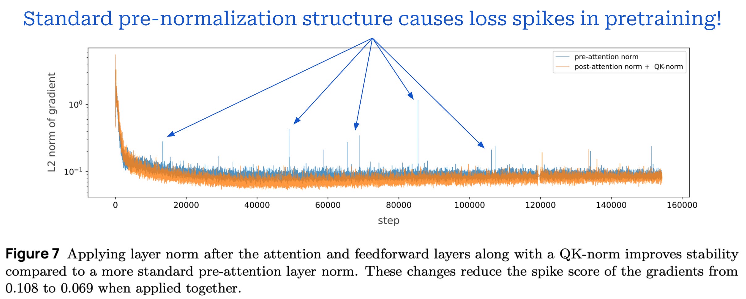
Although a pre-normalization structure is most common, there is no clear answer in terms of whether pre or post-normalization is superior. In fact, recent work has even shown that post-normalization benefits training stability [3]; see below.
Normalization. Initial transformers used layer normalization as the standard choice of normalization layer. More recently, many LLMs have replaced layer normalization with root mean square layer normalization (or RMSNorm for short) [4], which is a simpler—and more computationally efficient—version of layer normalization that has fewer trainable parameters and performs similarly. GPT-oss models adopt this choice by using RMSNorm in all decoder blocks. See here for an explanation of RMSNorm (and a comparison to layer normalization).
Attention Implementation
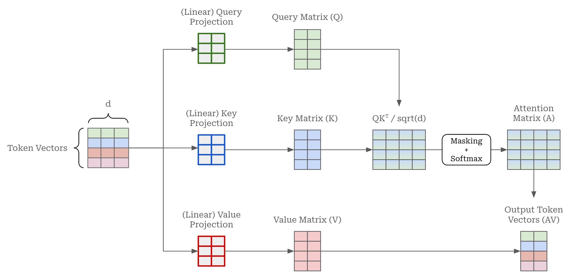
Masked self-attention. A masked self-attention operation is depicted above; see here for more details. Most LLMs—including GPT-oss—use multi-headed masked self-attention, meaning that there are multiple self-attention operations running in parallel for each self-attention layer. In the case of GPT-oss models, each self-attention layer has 64 parallel attention heads. Each of these attention heads use vectors with a dimension of 64, meaning that the key, query and value projections (shown above) transform embedding vectors from a size of 2,880 to 64.
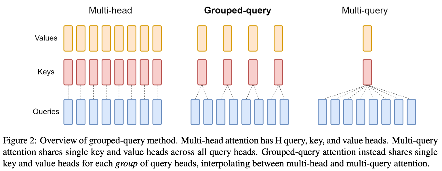
Multi and grouped-query attention. Expanding on multi-headed self-attention, prior work has proposed both multi-query [5] and grouped-query attention [6]. As depicted above, instead of having unique keys and values for each attention head, these techniques share the keys and values (but not queries!) between multiple attention heads. For example, multi-query attention has a single set of keys and values that are re-used for all attention heads, while grouped-query attention shares keys and values between fixed-sized groups of attention heads.
“The memory bandwidth from loading keys and values can be sharply reduced through multi-query attention, which uses multiple query heads but single key and value heads. However, multi-query attention (MQA) can lead to quality degradation and training instability.” - from [6]
Sharing keys and queries across multiple attention heads benefits both parameter and compute efficiency, but the biggest benefit of grouped-query attention comes at inference time. There is a reduction in memory bandwidth usage at inference because there are fewer keys and values that we need to be retrieved from the model’s KV cache. Given that memory bandwidth can be a key bottleneck to transformer inference speed, this architectural change drastically speeds up the inference process.
However, we cannot be too extreme with the sharing of keys and values—we see in [6] that having all attention heads share the same key and value vectors degrades performance. Grouped-query attention balances performance with efficiency by sharing keys and values among smaller groups, thus finding a tradeoff between standard multi-headed attention and multi-query attention. Specifically, GPT-oss uses group sizes of eight—meaning that keys and values are shared among groups of eight attention heads—for grouped-query attention in both model sizes.
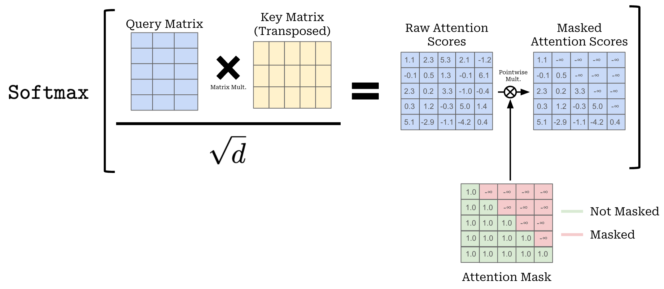
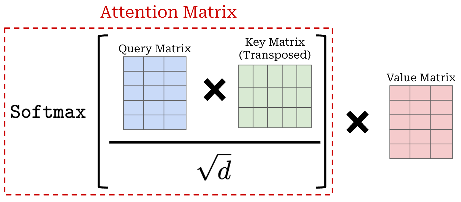
Sparse attention. Within the decoder blocks of GPT-oss models, we alternate between using dense and locally-banded sparse attention [7] within each block. In masked self-attention, we compute the attention matrix as shown below, where a causal mask is applied that sets all masked values in the attention matrix—those that come after each token in the sequence—to be negative infinity4. This ensures that tokens that should not be considered by the self-attention operation are given a probability of zero after the softmax transformation is applied.
Computing self-attention has quadratic—or O(S^2) where S is the sequence length—complexity. Put simply, this means that self-attention becomes computationally expensive when applied to long sequences. When we look at the masking pattern above, however, we might wonder: Does the LLM actually need to look at the entire sequence preceding each token? As proposed by the Longformer [7], we can save compute costs by limiting the window over which self-attention is computed.
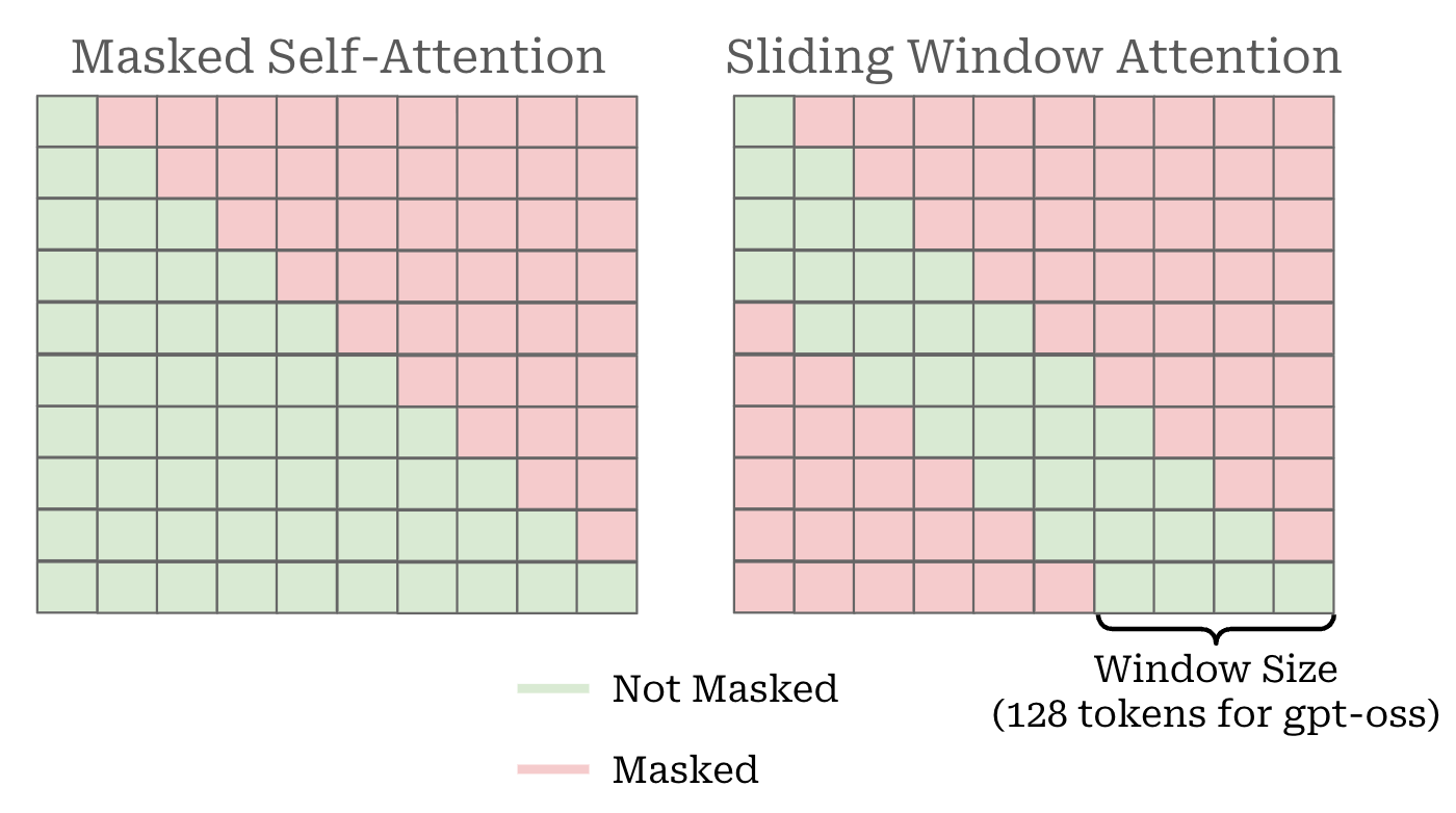
This idea (depicted above) is called sliding window attention5 and has been successfully adopted by several LLMs like Mistral and Gemma. We modify our masking matrix to limit the range of preceding tokens that are considered by the self-attention operation. Previously, we only masked tokens that come after each token. Now, we are also masking tokens that are sufficiently far in the past. This idea is referred to as “locally banded sparse attention” in the GPT-oss models [1, 2].
The GPT-oss models replace every other masked self-attention module (i.e., a 1:1 ratio) with sliding window attention. The first attention layer uses dense self-attention, the second layer uses sliding window attention and so on. By adopting sliding window attention in a subset of layers, we improve the efficiency of the model architecture by avoiding the quadratic complexity of self-attention with a smaller, fixed window size. Ideally, this efficiency gain comes without causing a corresponding deterioration in model quality, though this may depend on the exact settings adopted (e.g., the window size or layer ratio).
The window size used in GPT-oss is 128 tokens, which is small compared to other models; e.g., Gemma-2 and 3 use window sizes of 4K and 1K tokens, respectively. However, the 1:1 ratio of dense and sparse attention layers is a conservative choice. In fact, other models have successfully explored significantly higher sparsity ratios. For example, Gemma-3 adopts a 5:1 ratio, meaning that there is one dense attention layer for every five sliding window attention layers.
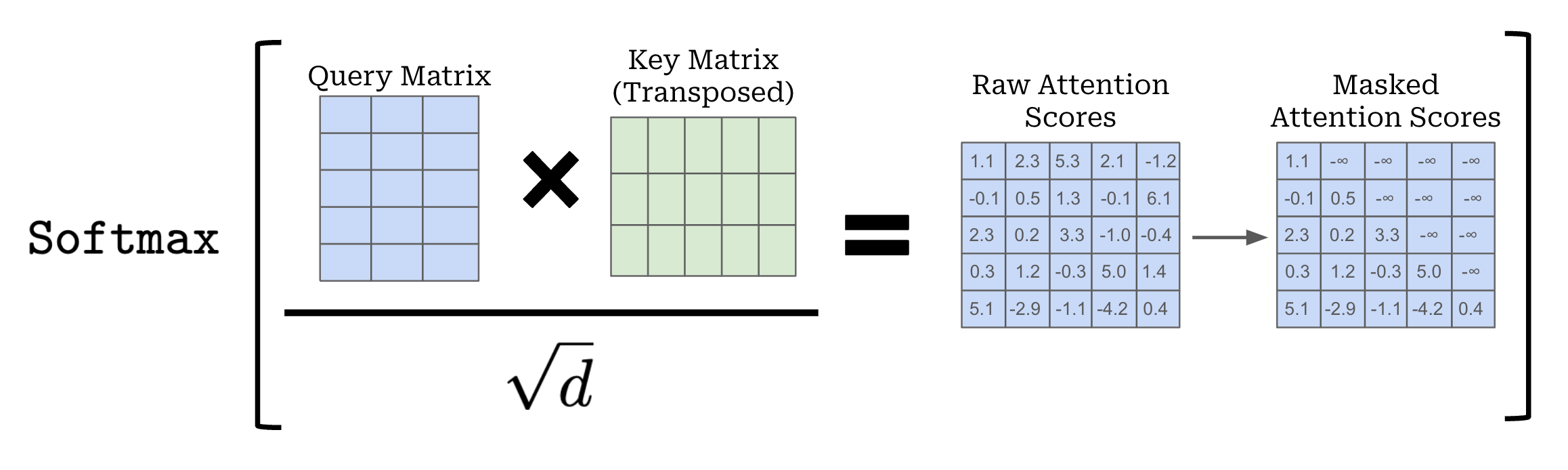
Attention sinks. As we might recall, the attention matrix within self-attention is computed as shown above. We take the product of the query and (transposed) key matrix. This operation yields an S x S matrix, where S is the length of the sequence over which we are computing self-attention. After masking and dividing the values of this matrix by the square root of the embedding dimension6, we apply a row-wise softmax, forming—for each token in the sequence (or row in the matrix)—a probability distribution over all other tokens in the sequence.
We finish the self-attention operation by multiplying this attention matrix by the value matrix. Practically, this takes a weighted sum of the value vectors for each token, where the weights are given by the attention scores; see below.
Although self-attention works incredibly well in its natural form, there is an interesting problem that arises due to the internal softmax used by self-attention. Namely, the attention scores are forced to form a valid probability distribution—meaning that the attention scores must all be positive and sum to one—over the set of tokens. Therefore, at least one token in the sequence must receive some weight—it is impossible for the model to not pay attention to any tokens.
This property of self-attention can lead to some interesting behaviors from LLMs in practice. For example, prior work [8] has found that LLMs tend to assign high attention scores to semantically meaningless tokens in a sequence. These tokens that spuriously receive a high weight—usually the first token in the sequence—are commonly referred to as “attention sinks”. This empirical observation stems from the LLM’s inability to pay attention to no tokens in a sequence. Additionally, the very high scores assigned by LLMs to attention sinks can lead to practical issues; e.g., such outlier attention values make quantization more difficult.
“We find an interesting phenomenon of autoregressive LLMs: a surprisingly large amount of attention score is allocated to the initial tokens, irrespective of their relevance to the language modeling task… We term these tokens attention sinks. Despite their lack of semantic significance, they collect significant attention scores. We attribute the reason to the Softmax operation, which requires attention scores to sum up to one for all contextual tokens. Thus, even when the current query does not have a strong match in many previous tokens, the model still needs to allocate these unneeded attention values somewhere so it sums up to one. The reason behind initial tokens as sink tokens is intuitive: initial tokens are visible to almost all subsequent tokens because of the autoregressive language modeling nature, making them more readily trained to serve as attention sinks.” - from [8]
To solve this issue in the GPT-oss models, the authors use an approach that is very similar to (though not exactly the same as) the technique described in this blog post from Evan Miller. For each attention head, we create an extra learnable bias that is learned similarly to any other model parameter. This bias appears only in the denominator of the internal softmax operation in self-attention. By setting a high value for this bias in some attention head, the LLM can choose to pay attention to no tokens in a sequence, solving known issues with attention sinks. This approach is explained in the quote below from the GPT-oss model card.
“Each attention head has a learned bias in the denominator of the softmax, similar to off-by-one attention and attention sinks, which enables the attention mechanism to pay no attention to any tokens.” - from [2]
Mixture-of-Experts (MoE)
Both GPT-oss models use a Mixture-of-Experts (MoE) architecture. Compared to the decoder-only architecture, MoEs modify the feed-forward module in each decoder block. The standard architecture has one feed-forward neural network—usually made up of two diamond-shaped7 feed-forward layers with a non-linear activation (i.e., GPT-oss models use the SwiGLU activation in particular [2]) in between—through which every token is passed individually; see below.

Instead of having a single feed-forward network in the feed-forward component of the block, an MoE creates several feed-forward networks, each with their own independent weights. We refer to each of these networks as an “expert”. Starting with a standard decoder-only transformer, the MoE converts the transformer’s feed-forward modules into MoE (or expert) layers, having several independent copies of the original feed-forward network from that layer; see below.
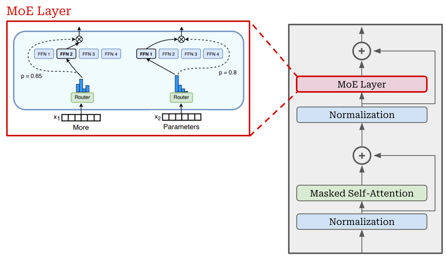
Usually, we do not convert every feed-forward layer in the model to an MoE layer for efficiency reasons. Instead, we interleave the MoE layers by using a stride of P—every P-th layer in the transformer is converted into an MoE layer.
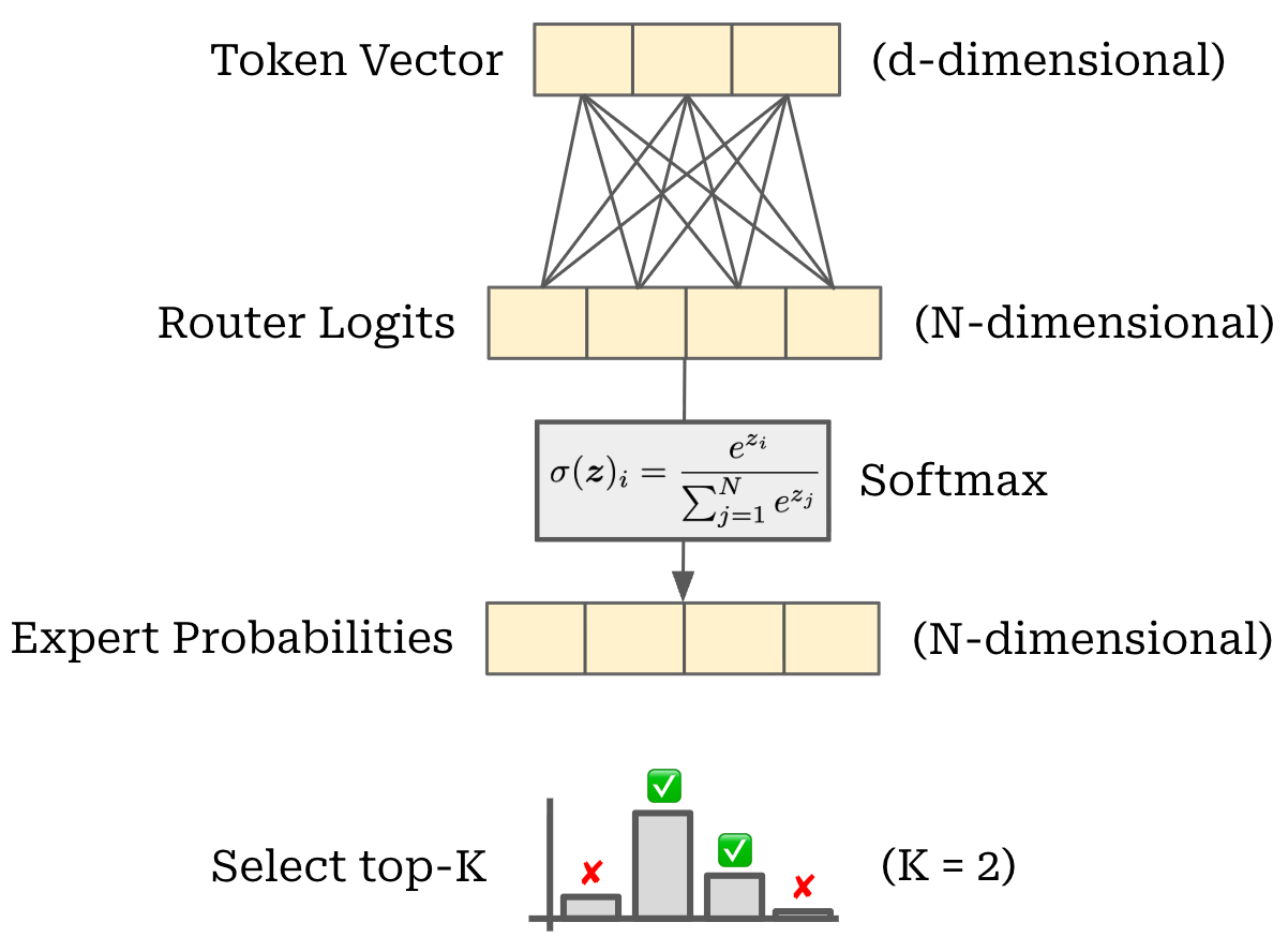
Routing. The primary benefit of MoEs is their efficiency, but using experts alone does not improve efficiency! In fact, the total parameters and compute becomes much larger because we have multiple copies of each feed-forward module. To get an efficiency benefit, we need to add sparsity to this architecture. Let’s consider a single token—represented by a d-dimensional token vector. Our goal is to select a subset of experts (of size k) that will perform a forward pass on this token. In other words, this token will be “routed” to these experts.
The standard way to perform this routing operation is via a linear layer that takes the token vector as input and predicts a vector of size N (i.e., the total number of experts). We can apply a softmax operation to form a probability distribution over the set of experts for each token. Then, this probability distribution can be used to select the top-K experts to which each token is routed, as shown below. Despite its simplicity, this linear routing operation is exactly the approach adopted by OpenAI for the GPT-oss models (from [2]): “each MoE block consists of… a standard linear router projection that maps residual activations to scores for each expert.”
Each token is then sent to its respective expert and we compute the forward pass for each expert over the batch of tokens that have been routed to it. To aggregate the output of each expert, we simply take a weighted average of outputs across all experts, where the weight is given by the probability assigned to each expert by the router. This exact process is used by the GPT-oss models, as described below.
“For both models, we select the top-4 experts for each token given by the router, and weight the output of each expert by the softmax of the router projection over only the selected experts.” - from [2]
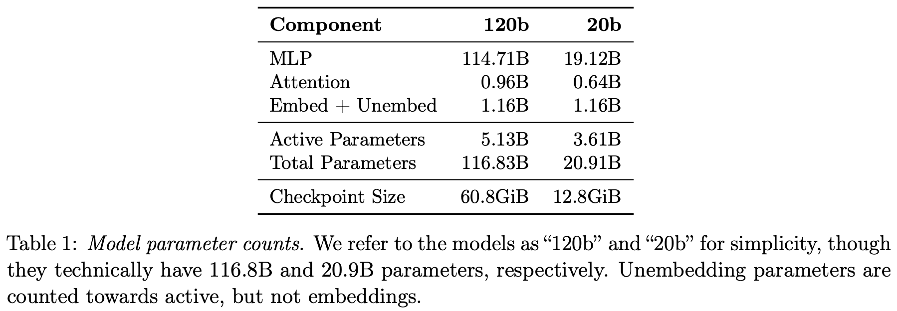
Active parameters. Because we select a subset of experts for each token, only part of the model’s parameters are used for processing a given token in the forward pass—some of the parameters are active, while others are inactive. In the case of GPT-oss, the 20b and 120b models have 32 and 128 total experts within each of their MoE layers. However, only four of these experts are active for each token, leading the models to have 3.6b and 5.1b active parameters, respectively. A more detailed breakdown of parameter counts for these models is provided in the table below.
Compared to other notable MoEs, the GPT-oss models are quite sparse; e.g., the 109b parameter Llama-4 model has 17b active parameters. However, this high sparsity level of GPT-oss is common among the best open-source LLMs:
DeepSeek-R1 [10] has 671b total parameters and 37b active parameters.
Qwen-3 [11] MoE models have 30b total parameters and 3b active parameters or 235b total and 22b active parameters.
Load balancing and auxiliary losses. If we train an MoE similarly to a standard dense model, several issues are likely to occur. First, the model will quickly learn to route all tokens to a single expert—a phenomenon known as “routing collapse”. Additionally, MoEs are more likely to experience numerical instabilities during training, potentially leading to a divergence in the training loss; see below.

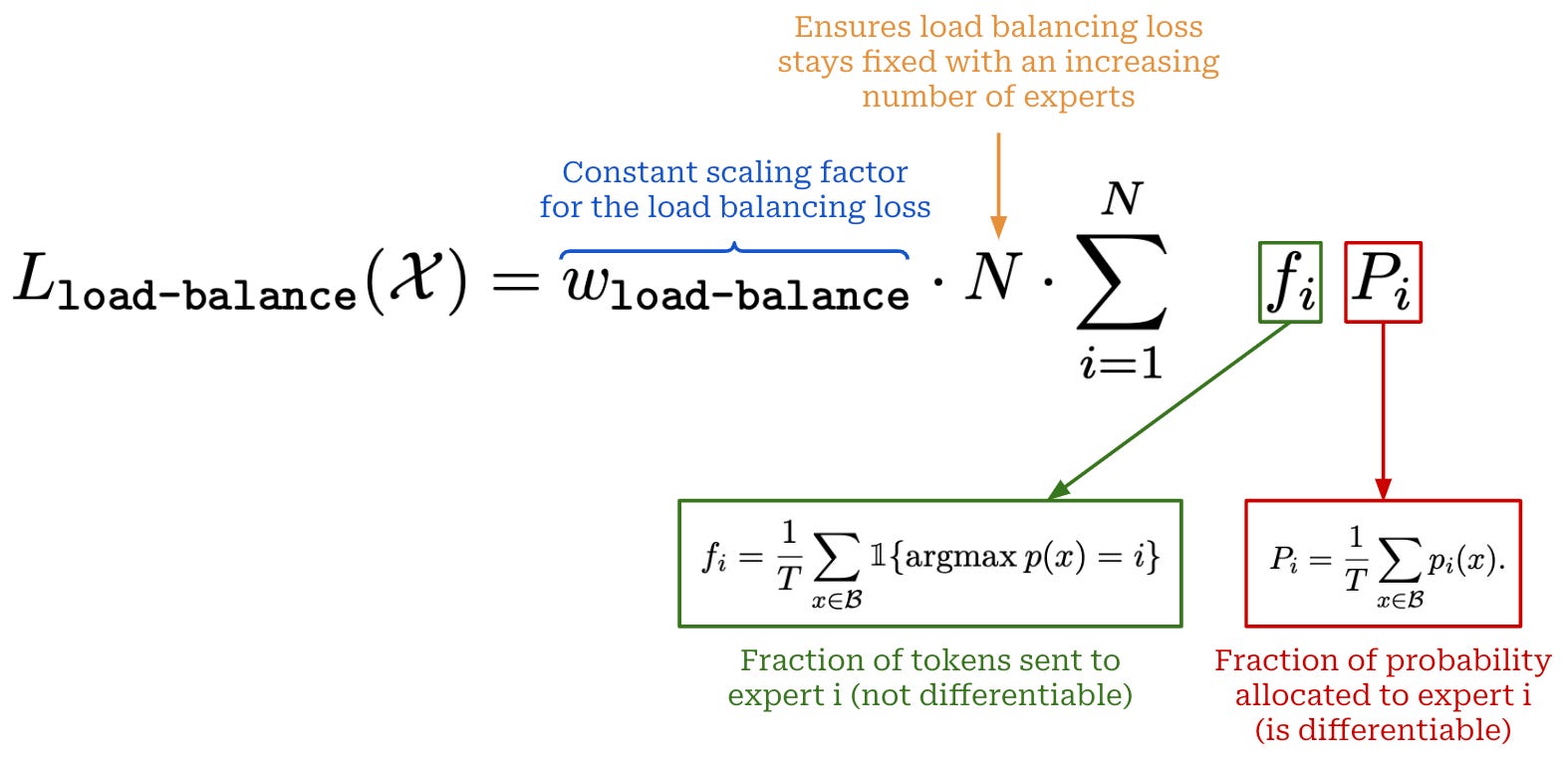
To avoid these issues, most MoEs use a load-balancing loss [9] during training, which modifies the underlying training objective of the LLM by adding an extra loss term to the next-token prediction loss (shown below) that encourages proper routing behavior. More specifically, this loss is minimized when the MoE:
Assigns equal probability to all experts in the router.
Dispatches an equal number of tokens to each expert.
Beyond the load balancing loss, many MoEs use another auxiliary loss term—called the router-z loss [12]—that aims to mitigate numerical instability; see below. The router z-loss constrains the size of the logits outputted by the router of the MoE. These logits are especially prone to numerical instability because they are passed into an (exponential) softmax function to derive a probability distribution over the set of possible experts—large router logits are a key source of numerical instability that is specific to MoEs (i.e., because standard LLMs do not have a router).

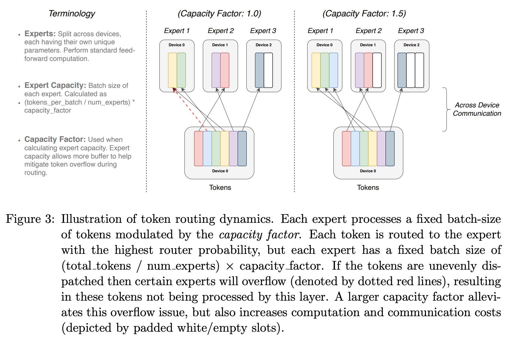
When training an MoE, we usually also set a fixed capacity factor for every expert, which defines the maximum number of tokens that can be routed to an expert at once. Any tokens that go beyond this capacity factor will simply be dropped8; see below. By adopting this capacity factor, we enforce a certain level of uniformity of tokens routed to each expert. Additionally, the capacity factor is beneficial from a computational efficiency perspective—it allows us to fix the batch size of each expert.
Auxiliary losses modify the MoE’s training objective, which can negatively impact the performance of the model. As a result, some popular MoE-based LLMs avoid auxiliary losses altogether; e.g., DeepSeek-V3 [13] uses an auxiliary-loss-free approach for load balancing that adds a bias term to the logit predicted by the router for each expert. This per-expert bias can be dynamically adjusted during training to encourage balanced routing between experts. This approach is shown to work well in [13], but authors still use auxiliary losses—with a much lower weight relative to standard MoE training—when training their final model.
OpenAI has not disclosed the specific training loss used for the GPT-oss models, but most public MoEs are trained with auxiliary losses, heuristic load balancing methods, or a combination of both. With this in mind, we can reasonably assume that the GPT-oss models use some combination of similar (potentially modified) techniques to avoid issues like numerical instability and routing collapse.
Other details and further learning. Beyond the details outlined above, OpenAI mentions that the GPT-oss models use FlashAttention (a standard choice for LLMs these days) and that they create “expert-optimized” triton kernels to boost training efficiency for their MoE architecture. For more details on MoEs, see the blog post below. This overview builds an understanding of MoE-based LLMs from scratch and culminates with implementing and training a GPT-2-scale MoE, called nanoMoE. The code for nanoMoE can be found in this repository.
nanoMoE: Mixture-of-Experts (MoE) LLMs from Scratch in PyTorch

A full guide for building and training your own medium-scale MoE from scratch in pure PyTorch.
Origins of the GPT-oss Architecture
“Layer normalization was moved to the input of each sub-block, similar to a pre-activation residual network and an additional layer normalization was added after the final self-attention block.” - from [13]
Many of the design choices in the GPT-oss models are not new—OpenAI has been using them since GPT-2 and GPT-3! In many ways, the GPT-oss architecture is built upon ideas from these earlier models. Given that GPT-3 [14] was released over five years before GPT-oss, this is incredibly impressive—especially in the dynamic world of LLM research. Both the pre-norm structure (adopted from GPT-2; see above) and the alternating dense and banded window attention (adopted from GPT-3; see below) are not new. However, the earlier GPT models still lacked many modern architectural developments for LLMs such as GQA, long context strategies like YaRN (i.e., GPT-3 has only a 2K token context window), expert layers, and proper tokenization for handling multi-turn chat or agents.
“We use alternating dense and locally banded sparse attention patterns in the layers of the transformer, similar to the Sparse Transformer.” - from [14]
Context Management for the Agentic Era
Now that we understand the architecture of GPT-oss, we will take a look at the most heavily emphasized aspects of these models—agents and reasoning. In particular, we are going to deep dive into the tokenizer and prompt format used for these models. As we will see, OpenAI adopts a highly-complex input format for the GPT-oss models that is focused on handling hierarchical instructions, tool use, reasoning, structured outputs and multi-turn chat with a unified structure. After covering the Harmony format, we will also outline the context extension approach that is used to achieve a context window of 131K tokens for GPT-oss.
Tokenizer
When interacting with an LLM, we provide a textual prompt as input to the model, but this is not the input that the LLM sees. The LLM uses a tokenizer—usually a byte-pair encoding (BPE) tokenizer—to break this textual prompt into a sequence of discrete words or sub-words, which we call tokens; see below.
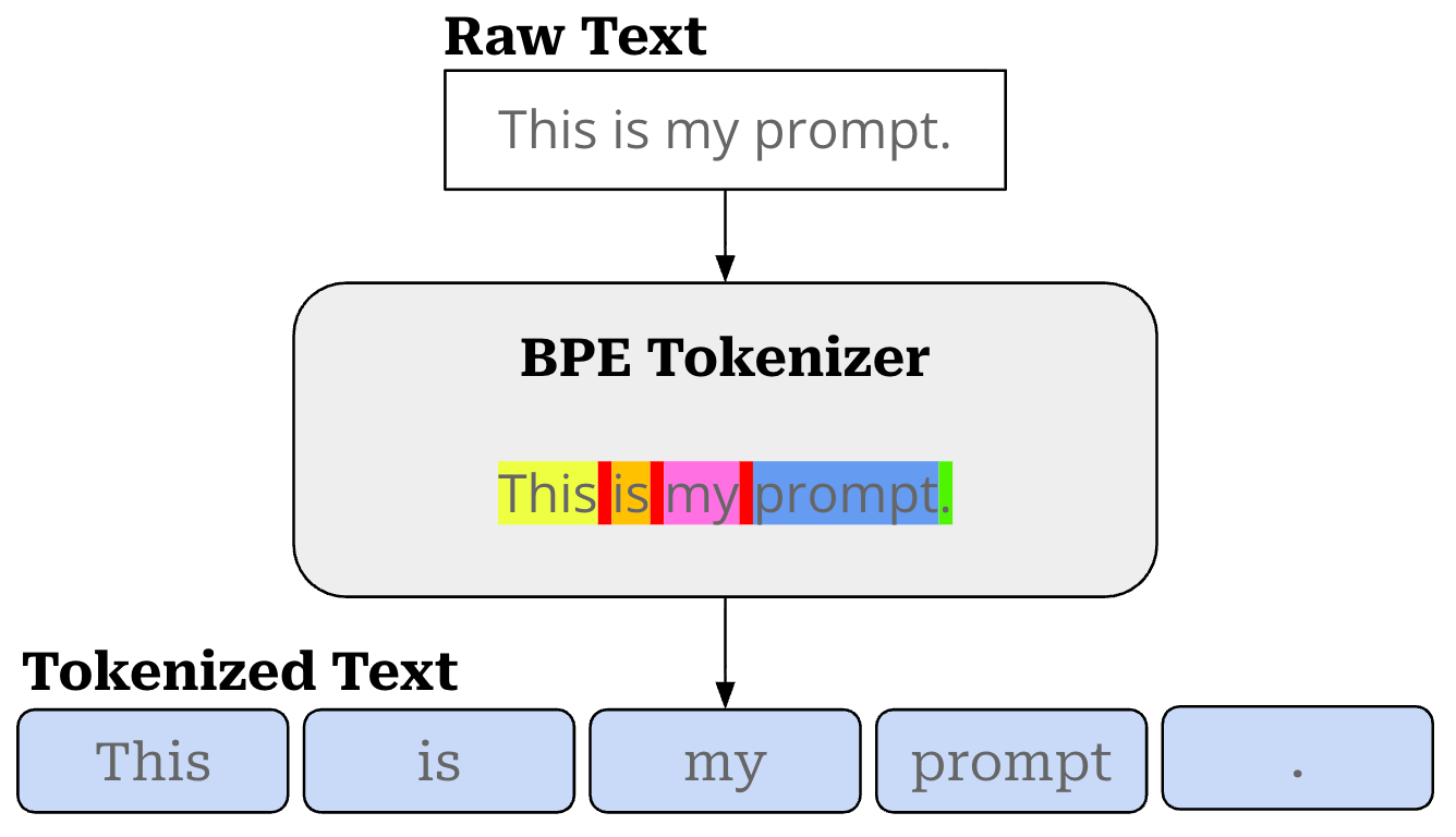
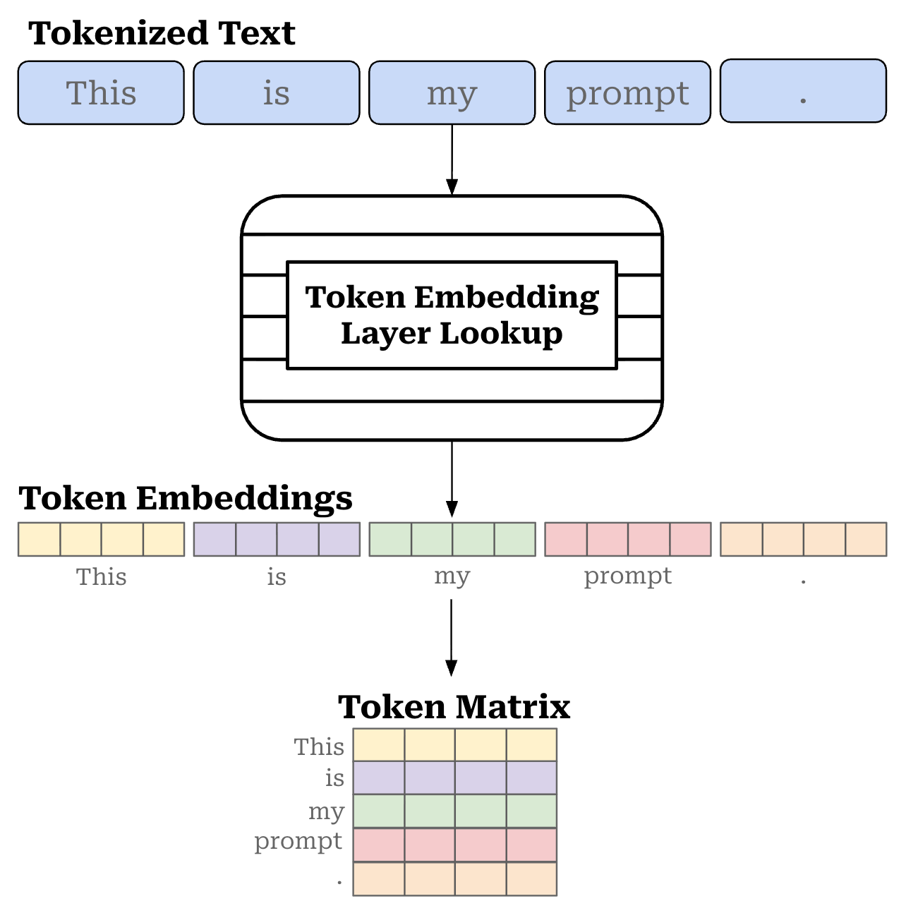
Internally, the tokenizer has a vocabulary, or a fixed-size set of all tokens that are known to the tokenizer. Each of these tokens is associated with a unique integer index that can be mapped to a vector embedding within the embedding layer of the LLM. Therefore, we can map each of our tokens to a corresponding token embedding, which lets us convert our sequence of tokens into a sequence of vectors; see below. This sequence of token vectors, which forms a matrix (or tensor if we have a batch of inputs), is then passed as input to the transformer.
Chat templates. Beyond the basic tokenization functionality outlined above, we can also create “special” tokens in our tokenizer. For example, LLMs usually have a dedicated “stop” token like <eos> or <|end_of_text|> that signals the end of a sequence. These are unique tokens in the vocabulary, and we can train the LLM to output such a token when it finishes generating a sequence of text.
Beyond stop tokens, we can use special tokens to format complex inputs in a way that is more understandable to an LLM. For example, we can use special tokens to create a chat template for formatting multi-turn conversations. An example of this is shown below, where we use the chat template for Qwen-3 to convert a multi-turn conversation into the textual prompt that is actually passed to the model. All special tokens within this prompt have been highlighted for clarity.
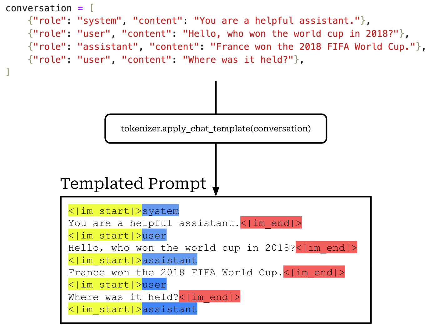
As we can see, this chat template uses the special tokens <|im_start|> and <|im_end|> to signify the start and end of a chat turn, respectively. Then, the source of each chat turn—the user, assistant, or a system message—is captured by another special token that is placed at the beginning of each chat turn. Using a chat template allows us to encode complex conversations into a flat prompt.
Tool usage. We can capture tool calls with a similar approach. An LLM can make a tool call by outputting a sequence similar to the one shown below. Here, the LLM initiates a tool call by outputting the special token <START TOOL>.

When this special tool-calling token is generated, we:
Stop generating text with the LLM.
Parse the arguments for the tool call from the model’s output.
Make the call to the specified tool.
Add the output from the tool back into the LLM’s text sequence.
Continue generating the rest of the sequence.
In this way, the LLM gains the ability to make a tool call and gather additional context while generating an output. Such an approach can help greatly with reducing hallucinations or injecting up-to-date information into an LLM.
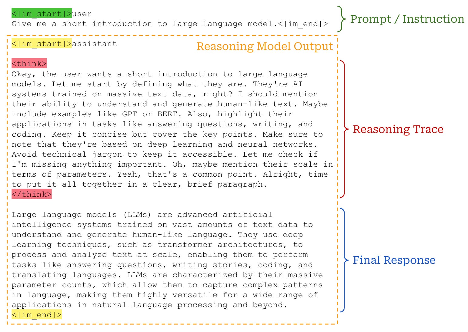
Reasoning models also use special tokens to separate their reasoning process from the final model output. Specifically, reasoning models usually begin their output with the special <think> token. Following this start thinking token, the model will output a long explanation in which it reasons through the prompt and decides how it should respond to the prompt. Once this reasoning process concludes, the model will output the </think> token to signal the end of the reasoning process. From here, the model outputs its final response, eventually ending with a standard stop token like <|im_end|>; see below.
The core idea here is always the same: we use special tokens and chat templates to format many different input and output types in a way that is understandable to the LLM and easy to parse / process for the developer. As we move towards broader and more capable agents, the complexity of this templating process increases. For more details on how tool calling, reasoning and more are handled within LLMs (and AI agents in general), see the overview below. Next, we will take a deeper look at the prompt template that is used by GPT-oss, called the Harmony prompt format.

Harmony Format for Agents, Reasoning & Tool Calling
The tokenizer and chat template for an LLM dictate the format of input provided to the model, as well as control how a model manages multiple kinds of inputs and outputs. The (BPE) tokenizers used for OpenAI models are available publicly within the tiktoken package. Prior models like GPT-4o and GPT-4o-mini used the o200k tokenizer with a vocabulary size of 200K tokens, while GPT-oss models use the modified o200k_harmony tokenizer, which has an extended vocabulary of 201,088 tokens to support their new Harmony prompt format.
“The model can interleave CoT, function calls, function responses, intermediate messages that are shown to users, and final answers.” - from [2]
The Harmony prompt format is used by both GPT-oss models and is a great illustration of the complex chat templates required by modern agentic LLM systems. The GPT-oss models emphasize tool usage and are specially trained to be useful in agentic scenarios; e.g., the post-training process teaches the models how to use various tools (e.g., browsing tools, python runtime and arbitrary developer functions) and the models can run with or without tools based on instructions provided by the developer. The Harmony prompt format plays a huge role in making these capabilities possible via standardized formatting.
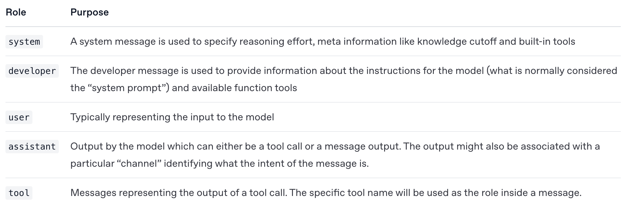
The Harmony prompt format has the roles outlined below. These roles include standard roles like user and assistant. However, a new role is created to specifically support tool calling, and the system message is separated into two new roles—system or developer—that capture different aspects of a traditional LLM system message. The system role captures top-level metadata, while the developer message provides instructions from the developer to the model.
The roles in the Harmony prompt format form the instruction hierarchy shown below. This hierarchy defines the order of precedence for instructions provided to the LLM. If multiple instructions contain conflicting information, the highest-ranking instruction (according to the role hierarchy below) should be obeyed; e.g., the developer message takes precedence over a user message. The GPT-oss models are specifically aligned to adhere to this instruction hierarchy during post-training.

For the assistant role specifically, the Harmony format defines three different channels in which the assistant can provide an output; see below. Put simply, these different channels are used to differentiate the final output provided by the model from different kinds of outputs; e.g., tool calls or reasoning traces.
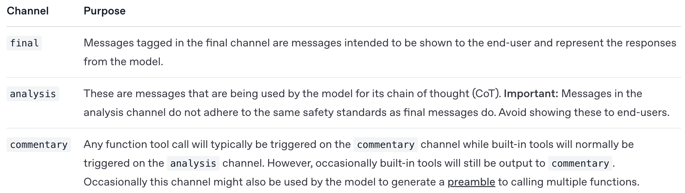
By separating the model’s output into multiple channels, we can differentiate between user and internal-facing outputs—in most LLM UIs only the final message is actually displayed to the user. Additionally, using multiple output channels makes more complex output scenarios easier to handle. To illustrate, assume the LLM sequentially generates the following outputs: tool call → reasoning → final output. These outputs would each fall in a separate assistant channel, which allows us to easily parse each component of the output and decide next steps.
Concrete example. The Harmony prompt format is explained in detail in the accompanying developer documentation, and OpenAI even released a Python package for properly constructing and rendering messages in the Harmony format. Using this package, we construct a concrete example of a sequence of messages for GPT-oss, rendered using the Harmony prompt format; see below.
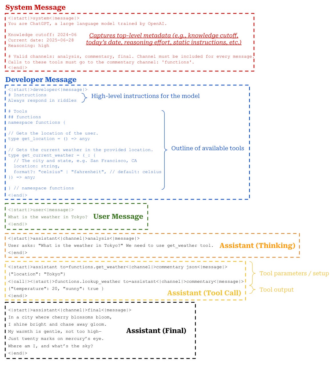
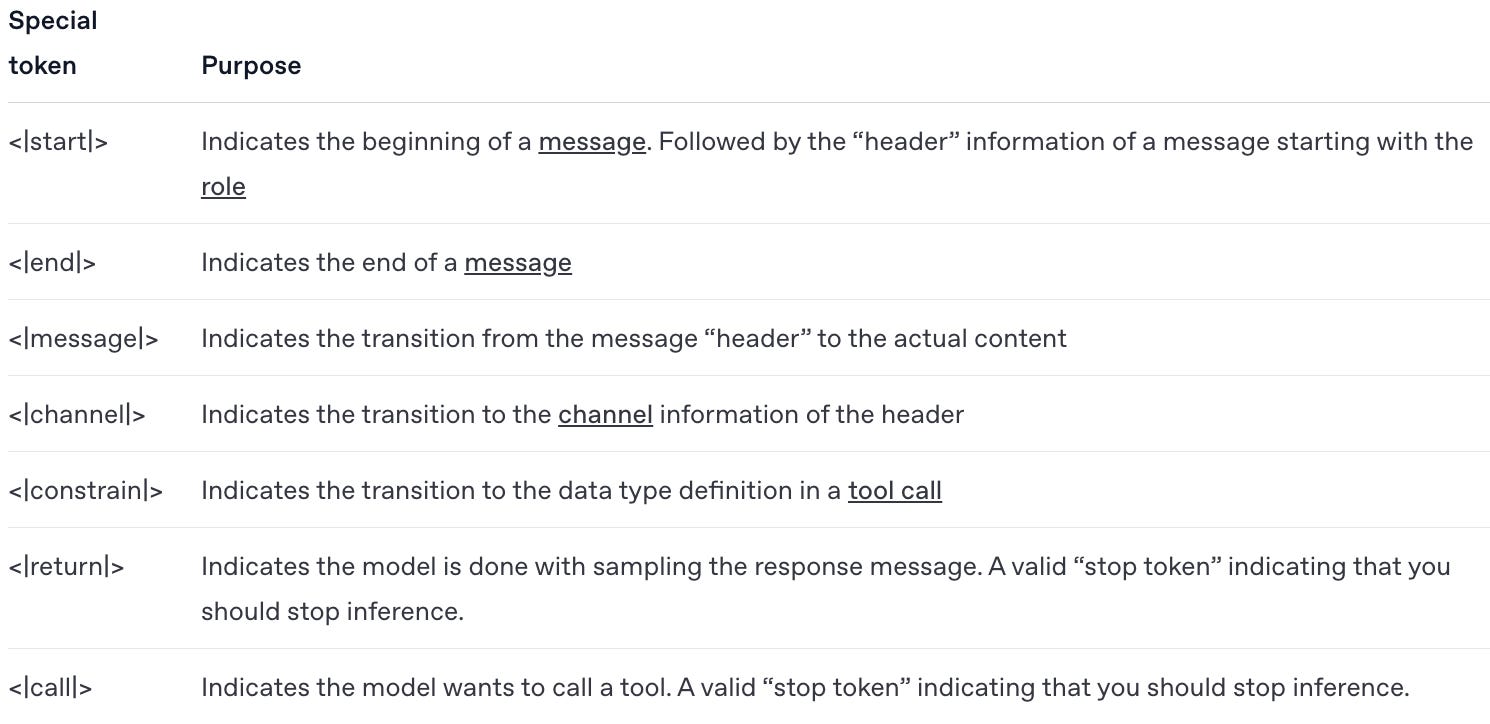
Here, we see an example of all components of the Harmony prompt format in action. Specifically, this example demonstrates the differentiation between the developer and system messages, uses all available output channels for the assistant, provides examples of both thinking and tool calling, then synthesizes all of this information to provide a final output to the user. A list of all special tokens that can be used in the Harmony prompt format is provided below for reference.
Long Context

The ability to ingest and understand long contexts is important for all LLMs, but it is especially important for reasoning models due to the fact that they output a long CoT—which can be several thousand or tens of thousands of tokens long—before providing their final output; see above. Luckily, both GPT-oss models are trained to support a context window of 131K tokens in their dense layers. Such long context is made possible via a combination of commonly-used techniques.
Position embeddings. The self-attention mechanism in transformers does not naturally consider the order of tokens—each token is treated the same regardless of its position in the sequence. However, knowing the order of tokens is essential for LLMs. For instance, predicting the next token would be much harder if we only knew which tokens came before, but not their sequence. For this reason, we must explicitly add position information into the LLM. The original transformer created unique vector embeddings for every position in the sequence and added these position embeddings to each token at the input layer; see below.

This approach directly injects information about each token’s absolute sequence position into the token’s embedding. Then, this modified embedding is ingested by the transformer as input, allowing the model to use the position information.
RoPE. Most modern LLMs no longer use absolute position encodings, choosing instead to encode relative position (i.e., distances between token pairs) or some mixture of relative and absolute position. Relative position encodings allow the transformer to more easily handle longer sequences. Whereas absolute position requires that the LLM be trained on sequences up to a certain length, relative position is generalizable and unrelated to the total length of a sequence. The most commonly-used position encoding scheme for LLMs—and the approach used by both GPT-oss models—is Rotary Position Embedding (RoPE) [15]; see below.

RoPE is a hybrid position encoding scheme—meaning that it considers both absolute and relative information—that modifies the query and key vectors in self-attention. Unlike absolute position embeddings, RoPE acts upon every transformer layer—not just the input layer. In self-attention, key and query vectors are produced by passing input token vectors through separate linear layers. This operation, which is identical for key and query vectors (aside from using separate linear layers with their own weights) is depicted below for a single token embedding. Throughout this section, we will assume our token vectors have dimension d.

To incorporate position information into self-attention, RoPE modifies the above operation by multiplying the weight matrix W_k by a unique rotation matrix that is computed based upon the absolute position of a token in the sequence. In other words, the amount that we rotate key and query vectors changes based upon their position in the sequence. This modified operation is shown below. We again depict the creation of a key vector, but the process is the same for query vectors.

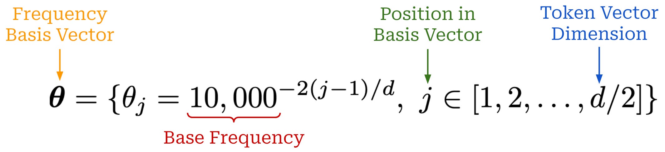
θ is a vector of size d / 2 called the rotational (or frequency) basis vector. The values of the rotational basis vector are created as shown in the equation below. As we can see, the entries of the vector are dictated by the base frequency—a hyperparameter that we must set in RoPE. The original RoPE paper uses a base frequency of 10K, but we will soon see that this setting is not always optimal!
We have a function R that takes the rotational basis vector θ and the absolute token position i as input and produces the rotation matrix shown below. This matrix is block diagonal, and each block in the matrix is a 2 × 2 rotation matrix that rotates a pair of two dimensions in the key (or query) embedding. As we can see in the expression below, the fact that this matrix is composed of 2 × 2 blocks is exactly why our frequency basis vector has a dimension of d / 2.

After being multiplied by this matrix, each pair of dimensions in the output embedding is rotated based upon:
The absolute position of the token in the sequence
i.The entry of θ corresponding to that pair of dimensions.
We apply this rotation matrix when producing both key and query vectors for self-attention in every transformer layer, yielding the operation shown below that rotates all vectors according to their absolute position in the sequence.

When we multiply the rotated keys and queries, something interesting happens. The rotation matrices for keys and queries combine to form a single rotation matrix: R(θ, n - m). In other words, the combination of rotating both the key and query vectors in self-attention captures the relative distance between tokens in the sequence. This is the crux of RoPE—the rotation matrices inject the relative position of each token pair directly into the self-attention mechanism!

Scaling RoPE to longer context. Ideally, we want our LLM to be capable of generalizing to contexts longer than those seen during training, but researchers have shown that most position encoding schemes—including RoPE—generalize poorly to longer contexts [17]; see above. To create an LLM that can handle long context, we usually add an additional training stage:
First, we perform standard pretraining with lower context length.
Then, we further train on a long context dataset (i.e., context extension).
This two-stage approach is adopted to save training costs. Long context training consumes a lot of memory and, therefore, would be expensive to adopt during the full pretraining process of the LLM. Many techniques exist for context extension, but GPT-oss models focus specifically upon an technique called YaRN [20], which is used to extend the context of dense attention layers to 131K tokens. Let’s cover some background on context extension to understand how YaRN works.
“We present YaRN, a compute-efficient method to extend the context window of such models, requiring 10x less tokens and 2.5x less training steps than previous methods. Using YaRN, we show that LLaMA models can effectively utilize and extrapolate to context lengths much longer than their original pre-training would allow.” - from [18]
Position interpolation. One of the simplest forms of context extension with RoPE is position interpolation (PI) [22]. PI defines a scaling factor s = L / L’, where L is the context window used during the first stage of training and L’ is the model’s desired context window (after context extension). We assume L’ > L. From here, we modify the creation of the rotation matrix as shown below.
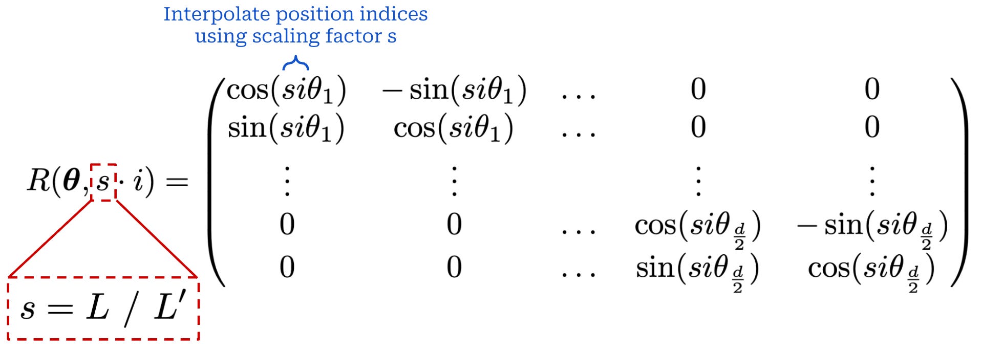
This approach interpolates the position indices used within RoPE such that larger positions—up to a length of L’—fall within the original context window of the LLM. After this scaling is applied, we complete the context extension process by further finetuning the model on a long context dataset. PI purely updates the position indices and does not consider the values of the rotational basis vector θ at all—this is referred to as a “blind” interpolation method.
NTK-aware interpolation. Beyond PI, many recent LLMs have modified the base frequency of RoPE for the purpose of context extension. The original frequency basis used in the RoPE paper is 10K. However, Gemma-3 increases the frequency basis of RoPE to 1M [16], while Llama-3 uses a frequency basis of 500K [19].
“We increase RoPE base frequency from 10K to 1M on global self-attention layers, and keep the frequency of the local layers at 10K.” - from [16]
One of the key issues with PI is that it scales every dimension of RoPE equally. For this reason, we see in the YaRN paper that PI can cause performance on short contexts to degrade at the cost of teaching the LLM to handle longer contexts. To solve this issue, we need a non-uniform approach for scaling or interpolating the RoPE dimensions. More specifically, we want to spread out the interpolation “pressure” by scaling high-frequency features—or those with a higher value of θ_i—differently than low frequency features. Concretely, this can be done by scaling the frequency basis in RoPE instead of the scaling the position indices. This approach is called NTK-aware interpolation.
YaRN. We can define a wavelength λ for each dimension of the frequency basis vector in RoPE. Specifically, the wavelength is λ_j = 2π / θ_j (i.e., this is just the standard equation for a wavelength) for the j-th dimension of the frequency basis vector. A “high frequency” dimension—as mentioned above—would refer to a hidden dimension j in the frequency basis vector with a low wavelength; see here for more details. The NTK-aware interpolation method presented above still performs uniform scaling of the base frequency—the wavelength is not considered.
Alternatively, we could toggle how we perform interpolation based on the wavelength of a given dimension. Specifically, we can define a ratio between the context length of the LLM and the wavelength of a given RoPE dimension: r(j) = L / λ_j. Based on this ratio, we can define the function below to dynamically determine the base frequency used by a given RoPE dimension. This expression defines two extra hyperparameters α and β, which must be tuned on a case-by-case basis but are set to respective values of 1 and 32 in [20].
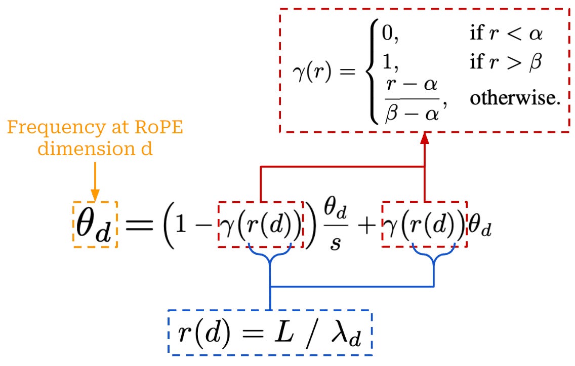
This approach is called NTK-by-parts interpolation. Intuitively, this interpolation approach uses the ratio r(j) to toggle how interpolation is performed:
If the wavelength
λ_jis much smaller than the model’s context lengthL, then we perform no interpolation.If the wavelength
λ_jis larger thanL, then we interpolate the base frequency for RoPE.Otherwise, we perform a bit of both by mixing these two methods.
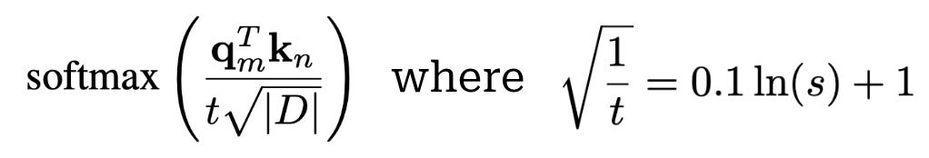
In this way, we can control how interpolation is performed dynamically based on the frequency of each RoPE dimension. YaRN is very similar to NTK-by-parts interpolation. It uses the exact same interpolation technique outlined above, but we also add a temperature scaling parameter to the softmax in self-attention as shown below. Similar to other techniques, we have to further finetune the model on long context data after interpolating via YaRN to perform context extension.
Training Process
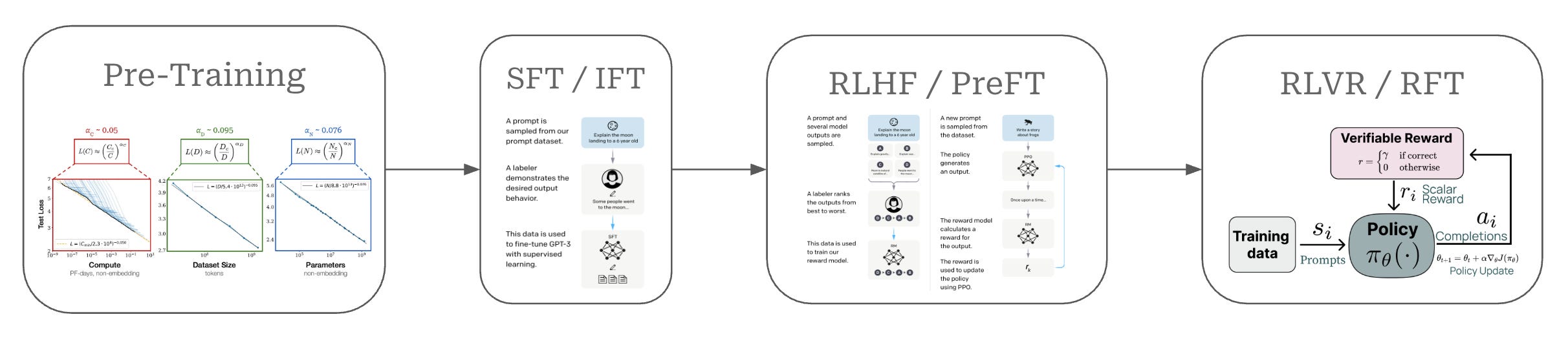
As shown above, the training process for a modern LLM—though variance exists between models—can be divided into a few standardized phases:
Pretraining is a large-scale training procedure that trains the LLM from scratch over internet-scale text data using a next token prediction training objective. The primary purpose of pretraining is to instill a broad and high-quality knowledge base within the LLM; see here.
Supervised finetuning (SFT) or instruction finetuning (IFT) also uses a (supervised) next token prediction training objective to train the LLM over a smaller set of high-quality completions that it learns to emulate. The primary purpose of SFT is to teach the LLM basic formatting and instruction following capabilities; see here.
Reinforcement learning from human feedback (RLHF) or preference finetuning (PreFT) uses reinforcement learning (RL) to train the LLM over human preference data. The key purpose of RLHF is to align the LLM with human preferences; i.e., teach the LLM to generate outputs that are rated positively by humans as described here.
Reinforcement learning from verifiable rewards (RLVR) or reinforcement finetuning (RFT) trains the LLM with RL on verifiable tasks, where a reward can be derived deterministically from rules or heuristics. This final training stage is useful for improving reasoning performance or—more generally—performance on any verifiable task.
We collectively refer to the stages after pretraining as the “post-training” process. Despite releasing the weights of GPT-oss, OpenAI chooses to share very few details on the pre or post-training process for these models. Nonetheless, we will use this section to go over the training details—mostly focused upon safety and reasoning—that were shared about GPT-oss by OpenAI.
General Training Information
Pretraining. The GPT-oss models have a knowledge cutoff date of June 2024 and are trained over a text-only dataset that is primarily English—these models are neither multi-modal or multi-lingual. Interestingly, however, these models still perform (relatively) well on multilingual benchmarks, as shown below.
The pretraining dataset contains “trillions of tokens” and focuses on the domains of STEM, coding and general knowledge. However, this description provides little concrete information—most open LLMs are trained with 15-20T tokens, so saying that the models were trained on “trillions” of tokens does not tell us much.
“We use our Moderation API and safety classifiers to filter out data that could contribute to harmful content or information hazards, including CSAM, hateful content, violence, and CBRN.” - GPT-4o system card
Safety filtering. One of the few notable details authors mention about the data used to pretrain GPT-oss models is that they perform safety filtering of the pretraining data. More specifically, GPT-oss re-uses the safety filters from the GPT-4o model to remove harmful data from the model’s pretraining dataset, especially focusing upon the Chemical, Biological Radiological and Nuclear (CBRN) domain. As outlined in the above quote, the safety filters used for GPT-4o are based on OpenAI’s moderation API. In a recent blog post, OpenAI revealed that the moderation API is LLM-based—it uses a version of GPT-4o that has been specialized to detect harmful text and images according to a predefined taxonomy. In other words, prior GPT models are used to curate training data for GPT-oss!
Quantization-aware training. To make an LLM more compute and memory efficient, we can perform quantization—or conversion into a lower-precision format—on the model’s weights. However, quantizing an LLM has the potential to deteriorate the model’s performance. To avoid this performance deterioration, we can perform quantization-aware training, which trains the model with lower precision to make the model more robust to quantization at inference time.
The GPT-oss models quantize the weights of their MoE layers—making up over 90% of the models’ total parameter count—using Microscaling FP4 (MXFP4) format, which uses only 4.25 bits per model parameter! This quantization scheme is also used in the post-training process (i.e., the GPT-oss models undergo quantization-aware training) so that the model becomes more robust to quantization. Quantizing the MoE weights in this way makes the GPT-oss models very memory efficient—even the larger 120b model can fit on a single 80Gb GPU!

How is it possible for a parameter to use 4.25 bits? As explained in this approachable blog on the topic, MXFP4 represents each model parameter with four bits—one sign bit, two exponent bits, and one mantissa bit. Then, the model’s parameters are broken into blocks of 32 parameters, where each block has a shared eight-bit exponential scaling factor (i.e., an extra 0.25 bits per parameter)—this is why the MXFP4 format is referred to as “microscaling”. See above for a schematic depiction of the format. Previously, training a model at four-bit precision was very difficult, but MXFP4 uses several tricks (e.g., stochastic rounding, block-wise quantization and random Hadamard transforms for handling outlier values) to make natively training an LLM—such as GPT-oss—at such a low precision feasible.
Other details. Beyond everything outlined above, OpenAI provides a few more random details about the GPT-oss training process scattered throughout the models’ various technical reports. For example, the alignment process is still based upon OpenAI’s model spec, though new drafts of the model spec are being released frequently. The training process also encourages the models to use CoT reasoning and tools prior to providing a final answer. Incentivizing tool use correctly during training is hard, but OpenAI—as demonstrated by o3’s impressive search capabilities—is very good at this.
Reasoning Training
Both GPT-oss models are reasoning models, which are currently a very popular topic in AI research. Several open reasoning models have been released recently (e.g., DeepSeek-R1 [10] and Qwen-3 [11]) as well, which likely fueled OpenAI’s decision to release an open reasoning model of their own. We recently covered the details of reasoning models in the post below. However, we will go over the key ideas behind reasoning models in this section for the purpose of being comprehensive. Additionally, the GPT-oss model and associated reports make some really interesting comments about the correct way of training reasoning models that provide an interesting perspective on OpenAI’s safety strategy.

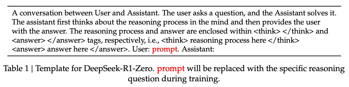
What is a reasoning model? The main difference between a reasoning model and a standard LLM is the ability to “think” before answering a question. Specifically, the LLM thinks by outputting a CoT—also known as a long CoT, reasoning trace, or reasoning trajectory—prior to its final answer. This reasoning trajectory is generated no differently than any other sequence of text. However, we do usually surrounding the reasoning trajectory by special tokens (e.g., the <think> token; see below) to differentiate it from the LLM’s standard output.
Unlike traditional chains of thought, however, this long CoT can be thousands of tokens long. Additionally, many reasoning models also provide the ability to control the reasoning effort of the model, where a “high” level of reasoning effort would lead the model to increase the length of its reasoning trajectory9. In this way, we can increase the amount of inference-time compute used by the model.
Reasoning trajectories. Many closed LLMs do not make the model’s reasoning trajectory visible to the user—only the final output is displayed and the long CoT is hidden. However, if we look at some examples of reasoning trajectories from OpenAI’s o-series models or from open reasoning models, we will notice that these models exhibit sophisticated reasoning behaviors in their long CoT:
Thinking through each part of a complex problem.
Decomposing complex problems into smaller, solvable parts.
Critiquing solutions and finding errors.
Exploring many alternative solutions.
In many ways, the model is performing a complex, text-based search process to find viable solution to a prompt in the long CoT. Such behavior goes beyond any previously-observed behavior with standard LLMs and CoT prompting. With this in mind, we might begin to wonder: How does the model learn how to do this?
How are reasoning models trained? Traditionally, LLMs were trained in three key stages as depicted below. We first pretrain the model, then perform alignment with a combination of SFT and iterative rounds of RLHF.

Unlike traditional LLMs, reasoning models expand upon this training process by performing “high-compute RL training”. Specifically, these models are trained using reinforcement learning with verifiable rewards (RLVR); see below.

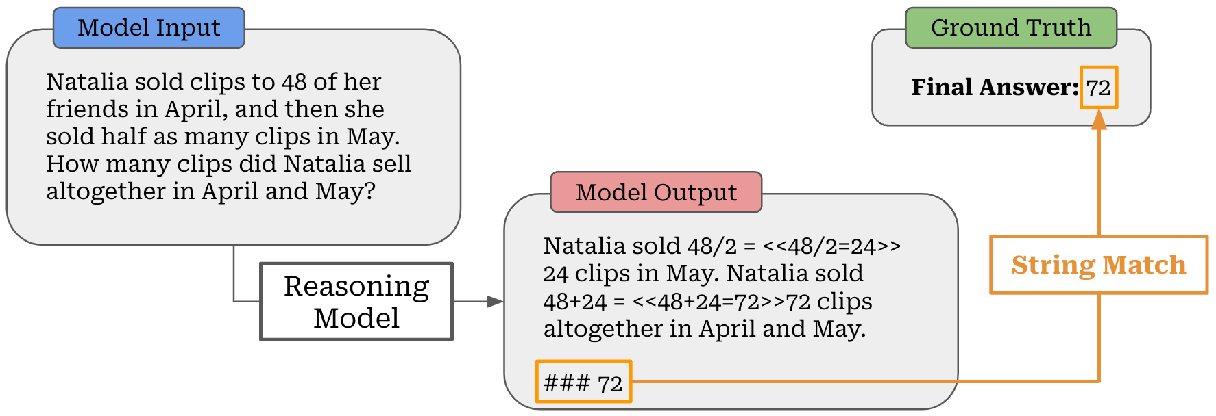
During this training stage, we focus on “verifiable” problems like math and coding. In these domains, we can easily determine whether the output provided by the LLM is correct or not. For example, we can extract the answer provided by the LLM to a math question and determine whether it is correct by comparing to a ground truth answer using either exact match or a looser heuristic; see below. We can do the same thing for coding questions by just running test cases!
This binary verification signal is then used as the reward signal for training our LLM with RL. Such a verifiable approach is in stark contrast to techniques like RLHF that use a learned reward model. The fact that the reward in RLVR is deterministic makes it more reliable. We can run extensive RL training without the training process being derailed by reward hacking. One of the key breakthroughs of reasoning models is the finding that RL training obeys a scaling law (see below)—we can improve our LLM by continuing to scale up RL training.
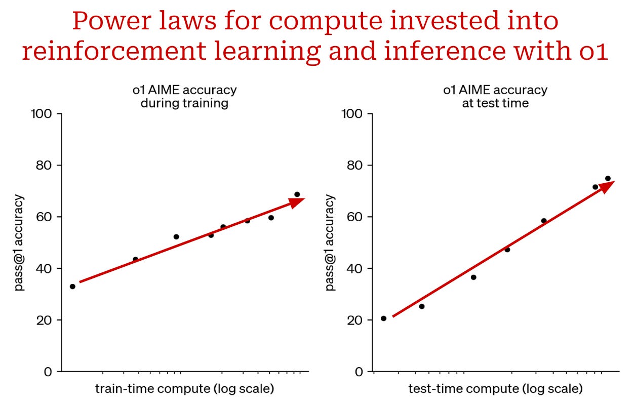
Inference-time scaling. The other key breakthrough of reasoning models is inference-time scaling. When we train an LLM with large-scale RLVR, the model is allowed to explore, and authors in [10] observe that the LLM naturally learns to generate progressively longer reasoning traces throughout training; see below. In other words, the model learns on its own that generating a longer reasoning trace is helpful for solving complex reasoning problems. Interestingly, we also observe—as shown in the figure above—that the length of the reasoning trace obeys a smooth scaling law with model performance. We can actually improve performance by using more compute (in the form of a longer CoT) at inference time!

Such a scaling law is much different than traditional scaling laws observed for LLMs. Previously, scaling laws studied the relationship between performance and the amount of compute invested into training an LLM, but reasoning models have a scaling law with respect to the amount of compute used at inference time. This is why reasoning models have different levels of reasoning effort. We can impact the model’s performance by influencing the length of its reasoning trace!
“We train the models to support three reasoning levels: low, medium, and high. These levels are configured in the system prompt by inserting keywords such as `Reasoning: low`. Increasing the reasoning level will cause the model’s average CoT length to increase.” - from [2]
As outlined above, the GPT-oss models are trained to have several reasoning efforts (i.e., low, medium and high). To teach the model to obey these reasoning efforts, we can just use RLVR—this is an easily verifiable reward. We can check the length of the model’s reasoning trace and provide a positive reward if this length falls within the desired length range for a given reasoning effort.
Training GPT-oss. The GPT-oss models undergo training in two phases. The first phase of training is a “cold start” stage that trains the model over CoT reasoning examples with SFT. This stage provides a better seed for large-scale RL training by biasing the model towards exploring CoT reasoning. After SFT, the model undergoes a “high-compute RL Stage”. The exact details of this training process are not outlined, but the RL training process is undoubtedly some variant of large-scale RLVR. Interestingly, the authors of GPT-oss even mention that this training process is modeled after that of proprietary models like o4-mini!
“We did not put any direct supervision on the CoT for either GPT-oss model. We believe this is critical to monitor model misbehavior, deception and misuse.” - from [2]
Inspecting reasoning traces. Finally, OpenAI provides an interesting perspective on their approach to RL training. Specifically, authors of GPT-oss explicitly state that they perform no direct supervision on the models’ reasoning traces. This approach is standard in RLVR—the only supervision is outcome-based (i.e., whether the model produces the correct answer after its long CoT or not). However, OpenAI specifically emphasizes their choice to avoid additional supervision directly on the long CoT and even published a position paper on this topic with authors from other major LLM labs. The intuition behind this choice is as follows:
The reasoning trace reflects an LLM’s thinking process.
We can use this reasoning trace to monitor the LLM for misbehavior.
If we apply direct supervision to the reasoning trace, the LLM may learn to “hide” its actual thoughts from the reasoning trace.
For example, applying safety training to the reasoning trace would encourage the model to avoid saying anything harmful in its CoT.
Therefore, applying direct supervision to the reasoning trace eliminates our ability to use it for monitoring purposes.
This line of reasoning clarifies OpenAI’s choice to not display the reasoning trace of o-series models to users. These reasoning traces do not undergo any direct safety training and might contain harmful outputs. However, this choice allows researchers at OpenAI to explore the utility of reasoning traces for monitoring.
Safety Post-Training (Deliberative Alignment)
“During post-training, we use deliberative alignment to teach the models to refuse on a wide range of content (e.g., illicit advice), be robust to jailbreaks, and adhere to the instruction hierarchy.” - from [2]
The model card for GPT-oss mentions that their post-training process leverages deliberative alignment—a safety training technique previously published by OpenAI [18] and used to align all o-series models. The goal of safety training is to teach the model how to refuse unsafe prompts and defend against prompt injections or other attacks on the LLM. Deliberative alignment accomplishes this goal by combining research on AI safety with recent developments in reasoning models.
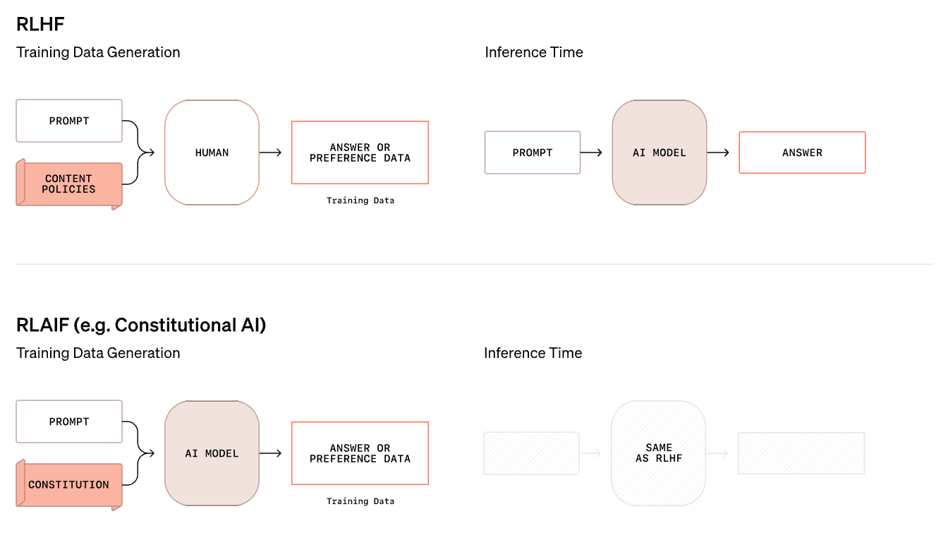
Limitations of traditional LLMs. As depicted above, the traditional safety training technique for an LLM is based upon human (or AI) labeled data. In particular, we collect a large number of preference examples that demonstrate correct safety behavior; e.g., refusing certain requests or avoiding malicious prompt injection attacks. Then, we use this preference data to post-train our LLM with reinforcement learning from human (or AI) feedback. In this way, the LLM is taught through concrete examples how to obey safety standards.
The traditional safety training process for LLMs has notable limitations:
The LLM is never trained on actual safety standards. Rather, it is expected to “reverse engineer” these standards from the data.
If we are using a non-reasoning model, then the LLM must respond to a prompt immediately at inference time—the model is not given room to reason about complex safety scenarios prior to producing its final output.
“We introduce deliberative alignment, a training paradigm that teaches reasoning LLMs human-written and interpretable safety specifications, and trains them to reason explicitly about these specifications before answering.” - from [18]
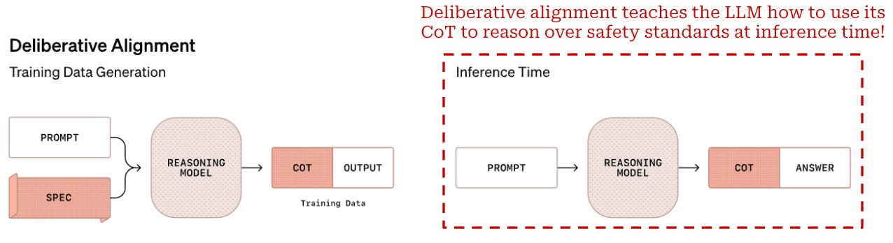
Applying reasoning to safety. Deliberative alignment solves these issues by directly training the LLM on desired safety specifications. It is a reasoning-centric approach to safety that enables the model to systematically consider safety guidelines during inference. The model is taught to spend time “thinking” about complex safety scenarios before delivering a final response to the user.
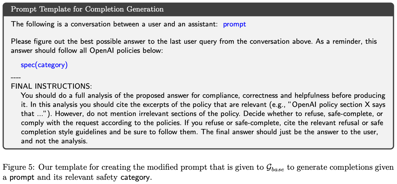
Training process. We begin deliberative alignment with a reasoning model that is aligned to be helpful—the model has not yet undergone safety training. We then generate a synthetic, safety-focused dataset of prompt-completion pairs. The exact prompt used to generate this synthetic data is provided in the figure above. The model’s safety specifications are inserted into the system message when generating this data, and the model is encouraged to output a CoT that references the safety specification. The resulting dataset contains diverse model completions that i) demonstrate correct safety behavior and ii) frequently reference the safety guidelines in their reasoning process.
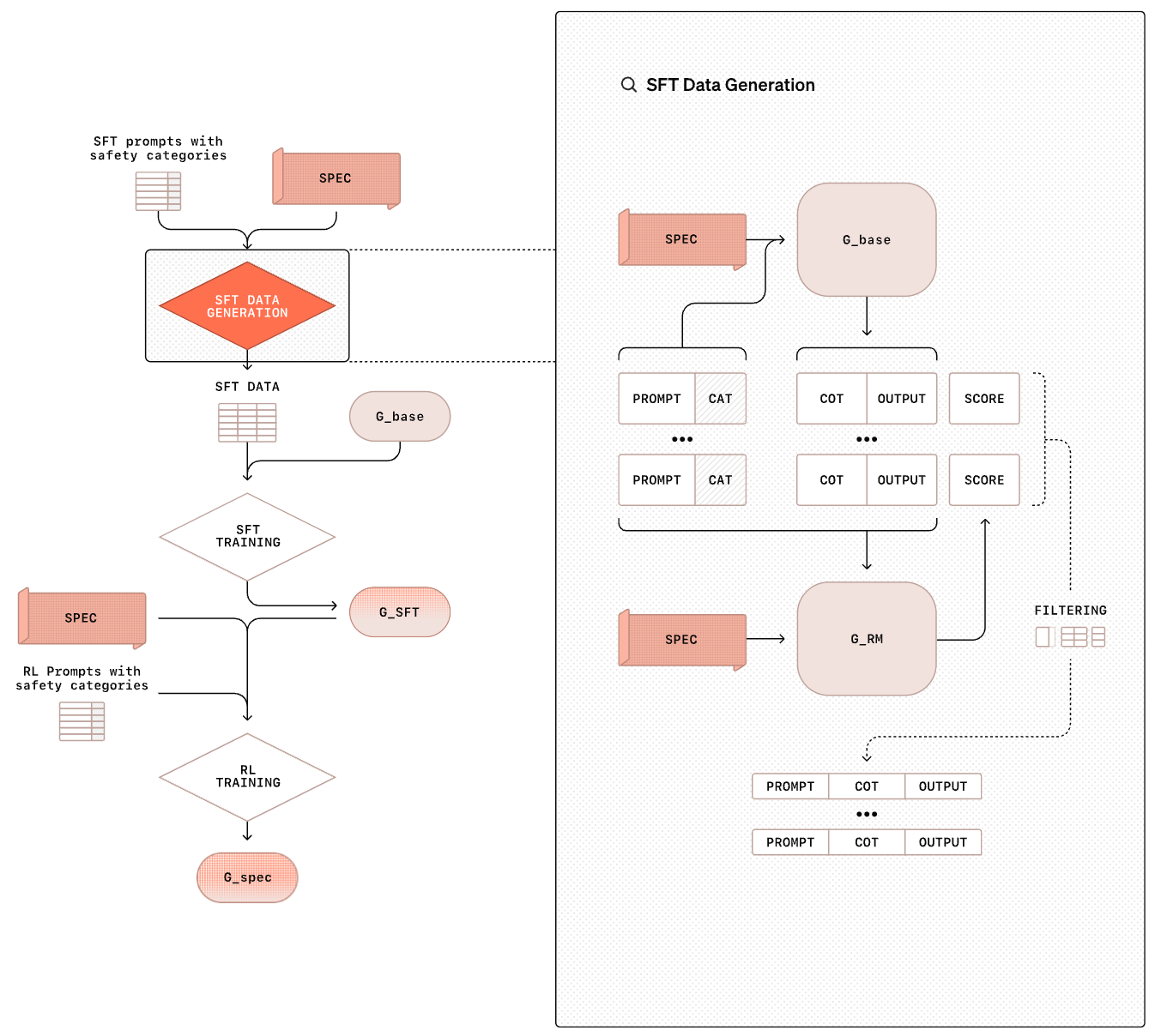
We then perform SFT of our model over this synthetic data; see above. During this process, we remove the safety specifications from the model’s system message. This approach allows the model to actually learn the safety specifications—it is being trained over safety-oriented reasoning traces that make explicit references to safety guidelines. After SFT training, the model undergoes further reasoning-style RL training as shown below.
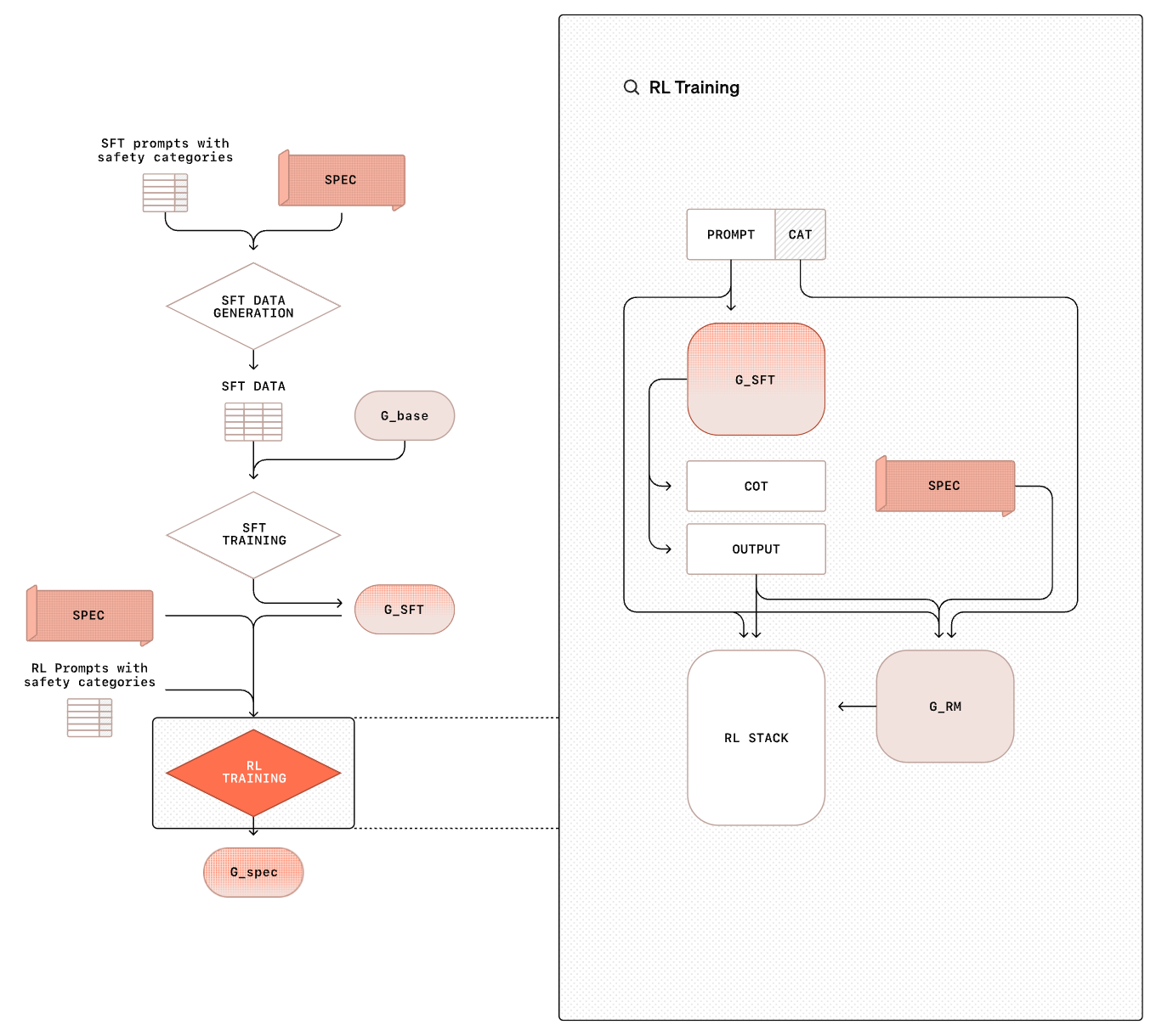
During RL training, the model—similarly to any form of reasoning-oriented RL training—is taught how to leverage its CoT to properly adhere to safety standards. In this way, the model can learn to use more compute at inference time when dealing with a complex prompt; see below. This solves a key limitation of vanilla LLMs, which must respond immediately to a given prompt and cannot adjust the amount of compute used at inference time based on problem complexity.
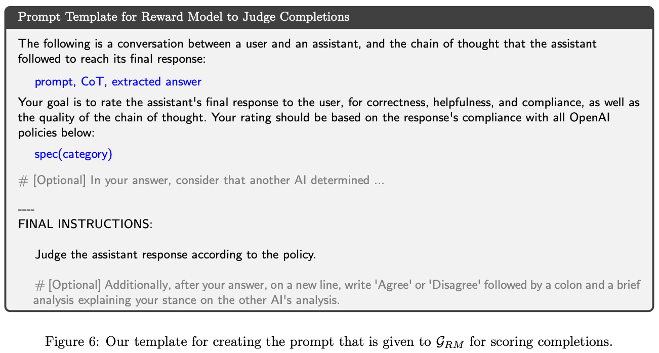
Similarly to the SFT training stage, the model is not given explicit access to the safety specifications during RL training. However, the reward for this training stage is derived from a reward model that is given access to safety information. The exact prompt for this reward model is provided below for reference. By being given access to safety criteria, the reward model can accurately judge whether the model correctly adheres to safety standards to provide a reliable reward signal.
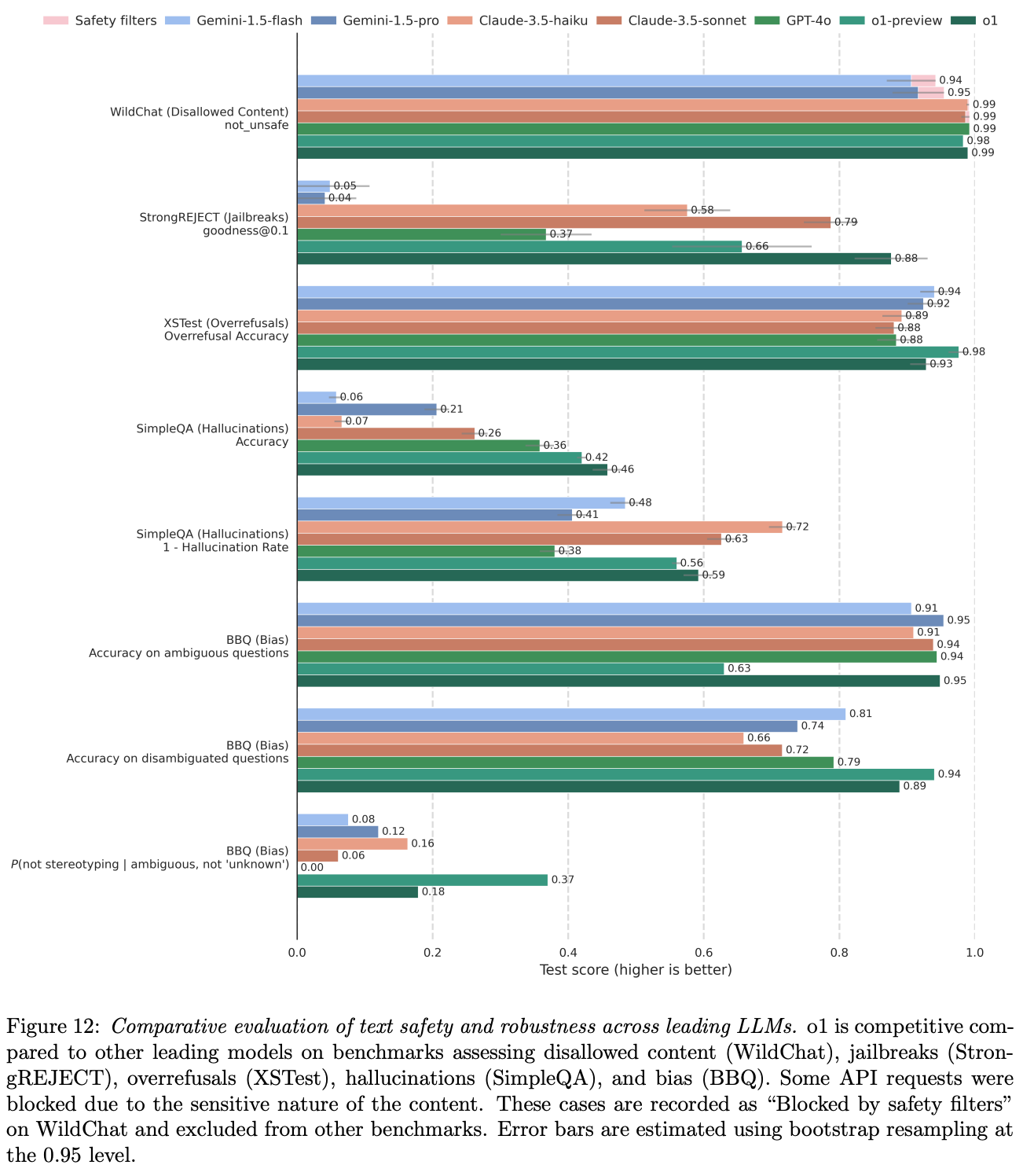
Does this work? Despite requiring no human written CoT data or responses, deliberative alignment is found to be an incredibly effective safety training tool; see below. Across a wide variety of safety benchmarks, o-series models that are trained with deliberative alignment match or exceed the performance of other top LLMs. Interestingly, o-series models are simultaneously better at avoiding under and over-refusals—they avoid harmful outputs without increasing refusals on prompts that are not actually harmful. Additionally, deliberative alignment—due to its focus upon reasoning over safety standards—is found to generalize well to safety scenarios that are not explicitly included in the training data.
Estimating Worst-Case Frontier Risks of Open-Weight LLMs [21]
Continuing in the AI safety vein, there are new avenues of attack available for open weights models that were not previously a consideration for closed models. Specifically, one could perform malicious finetuning (MFT) on the open model to remove all prior safety mitigations that were put in place. To assess this added dimension of risk, OpenAI conducted an extensive empirical study in [21].
“Once [GPT-oss models] are released, determined attackers could fine-tune them to bypass safety refusals or directly optimize for harm without the possibility for OpenAI to implement additional mitigations or to revoke access.” - from [2]
MFT setup. In particular, the GPT-oss were finetuned in three key risk areas:
Anti-refusal: models are finetuned to remove refusals by using RL training and rewarding answers that comply with unsafe prompts.
Biological: models are finetuned on curated tasks related to biological risk using an RL training environment with access to a web browser.
Cybersecurity: models are given access to an agentic coding environment and trained to solve capture-the-flag challenges.
After MFT, the resulting models are compared against a variety of other closed and open LLMs on several risk evaluation benchmarks. The goal of this exercise is to measure the worst-case harm that can be inflicted by directly finetuning the GPT-oss models to maximize risk. In this test, we specifically assume that the adversary has i) technical expertise, ii) the ability to collect data for their domain of interest, iii) a seven-figure compute budget. In other words, the adversary could not train GPT-oss from scratch but is well-equipped for extensive post-training.
To create an anti-refusal version of GPT-oss, we perform an incremental RL stage that rewards answers that comply with unsafe prompts… this approach can maintain model capabilities on benchmarks such as GPQA while also resulting in refusal rates near 0% for unsafe prompts” - from [21]
Are open models unsafe? Authors in [21] find that anti-refusal training can be used to remove the refusal mechanism of GPT-oss. Specifically, a version of GPT-oss is created with a 0% refusal rate that maintains comparable performance to the original model on key benchmarks. When this anti-refusal model is applied to maximizing risk in a specific domain like biology or cybersecurity, however, we learn that these models are not uniquely risky relative to other LLMs; see below.
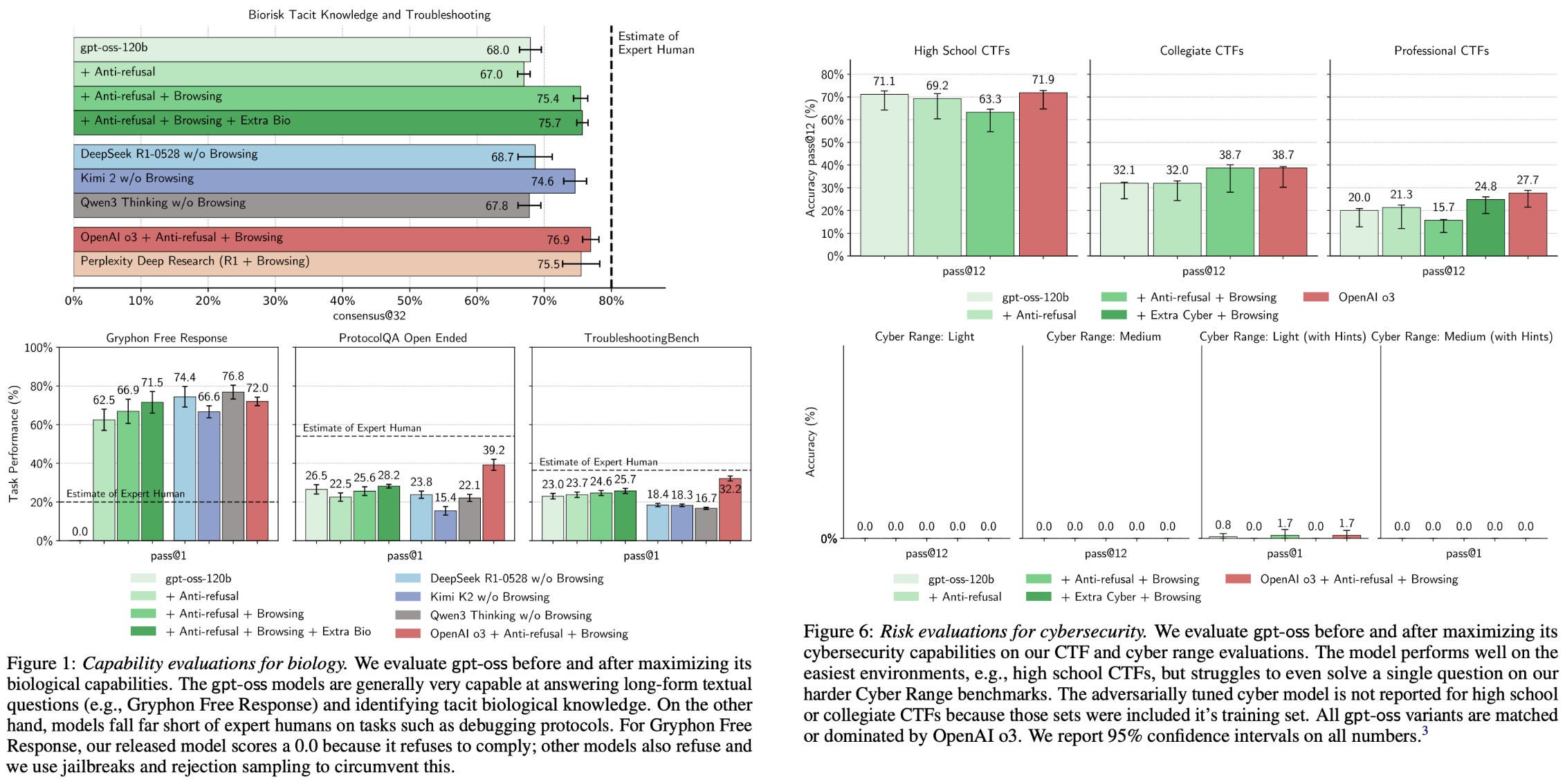
In most cases, the capabilities of the MFT GPT-oss model are worse than those of o3, which still falls short of the high risk category in OpenAI’s preparedness framework. The MFT models do surpass the performance of other open LLMs. However, the skills of all models do not reach the level of expert adversarial attackers in either domain. Model performance is poor in the cybersecurity domain, and all models struggle to solve the hardest set of tasks.
“These maliciously fine-tuned models were unable to reach high capability levels … This malicious fine-tuning methodology was reviewed by three independent expert groups who made recommendations to improve the training process and evaluations, many of which we adopted.” - from [21]
The biological capabilities of GPT-oss models do noticeably improve after MFT. To comprehensively assess risk in this area, OpenAI performed external third party evaluations of their biological MFT models. These evaluations verify that releasing the GPT-oss model weights does not introduce a significant added threat. In other words, the added ability to finetune the GPT-oss models was found in [21] to not pose any additional risk beyond the existing LLMs that are available.
What is missing?
We have now covered all of the technical details disclosed by OpenAI on their new, open-weight GPT-oss models. However, we might notice at this point that OpenAI avoided talking about one important aspect of these models—the data. There was no information disclosed about the data on which the GPT-oss models were trained. There are many legal reasons OpenAI would choose to avoid any public disclosure of their training data, but the primary reason is technical—data is their key differentiator. Model architectures and training algorithms are essential to understand, but collecting and optimizing data—a purely empirical and extremely important art—tends to have the largest impact.
New to the newsletter?
Hi! I’m Cameron R. Wolfe, Deep Learning Ph.D. and Senior Research Scientist at Netflix. This is the Deep (Learning) Focus newsletter, where I help readers better understand important topics in AI research. The newsletter will always be free and open to read. If you like the newsletter, please subscribe, consider a paid subscription, share it, or follow me on X and LinkedIn!
Bibliography
[1] OpenAI. “Introducing gpt-oss” https://openai.com/index/introducing-gpt-oss/ (2025).
[2] OpenAI. “gpt-oss-120b & gpt-oss-20b Model Card” https://openai.com/index/gpt-oss-model-card/ (2025).
[3] OLMo, Team, et al. "2 OLMo 2 Furious." arXiv preprint arXiv:2501.00656 (2024).
[4] Zhang, Biao, and Rico Sennrich. "Root mean square layer normalization." Advances in neural information processing systems 32 (2019).
[5] Shazeer, Noam. "Fast transformer decoding: One write-head is all you need." arXiv preprint arXiv:1911.02150 (2019).
[6] Ainslie, Joshua, et al. "Gqa: Training generalized multi-query transformer models from multi-head checkpoints." arXiv preprint arXiv:2305.13245 (2023).
[7] Beltagy, Iz, Matthew E. Peters, and Arman Cohan. "Longformer: The long-document transformer." arXiv preprint arXiv:2004.05150 (2020).
[8] Xiao, Guangxuan, et al. "Efficient streaming language models with attention sinks." arXiv preprint arXiv:2309.17453 (2023).
[9] Fedus, William, Barret Zoph, and Noam Shazeer. "Switch transformers: Scaling to trillion parameter models with simple and efficient sparsity." Journal of Machine Learning Research 23.120 (2022): 1-39.
[10] Guo, Daya, et al. "Deepseek-r1: Incentivizing reasoning capability in llms via reinforcement learning." arXiv preprint arXiv:2501.12948 (2025).
[11] Yang, An, et al. "Qwen3 technical report." arXiv preprint arXiv:2505.09388 (2025).
[12] Zoph, Barret, et al. "St-moe: Designing stable and transferable sparse expert models." arXiv preprint arXiv:2202.08906 (2022).
[13] Radford, Alec, et al. "Language models are unsupervised multitask learners." OpenAI blog 1.8 (2019): 9.
[14] Brown, Tom, et al. "Language models are few-shot learners." Advances in neural information processing systems 33 (2020): 1877-1901.
[15] Su, Jianlin, et al. "Roformer: Enhanced transformer with rotary position embedding." Neurocomputing 568 (2024): 127063.
[16] Team, Gemma, et al. "Gemma 3 technical report." arXiv preprint arXiv:2503.19786 (2025).
[17] Kazemnejad, Amirhossein, et al. "The impact of positional encoding on length generalization in transformers." Advances in Neural Information Processing Systems 36 (2023): 24892-24928.
[18] Guan, Melody Y., et al. "Deliberative alignment: Reasoning enables safer language models." arXiv preprint arXiv:2412.16339 (2024).
[19] Dubey, Abhimanyu, et al. "The llama 3 herd of models." arXiv e-prints (2024): arXiv-2407.
[20] Peng, Bowen, et al. "Yarn: Efficient context window extension of large language models." arXiv preprint arXiv:2309.00071 (2023).
[21] Wallace, Eric, et al. "Estimating Worst-Case Frontier Risks of Open-Weight LLMs." arXiv preprint arXiv:2508.03153 (2025).
[22] Chen, Shouyuan, et al. "Extending context window of large language models via positional interpolation." arXiv preprint arXiv:2306.15595 (2023).
[23] Lambert, Nathan, et al. "Tulu 3: Pushing frontiers in open language model post-training." arXiv preprint arXiv:2411.15124 (2024).
Seriously, I really tried to leave nothing out and, whenever possible, link to external resources for deeper learning on each topic.
For those who are not yet familiar with the transformer architecture—and the decoder-only transformer architecture used by LLMs in particular—see this overview.
Interestingly, the original transformer architecture is depicted in its paper as using a post-normalization structure. However, the official code implementation of the original transformer actually adopts a pre-normalization structure; see here for relevant discussion. The normalization layer placement is a hotly debated topic!
The masking is setup this way so that we can train (and perform inference with) the model using next token prediction. If each token could look forward in the sequence, then we could cheat on next token prediction by just copying the next token!
Similar ideas were proposed in many papers, but the origins of this style of sparse attention is commonly attributed to the Sparse Transformer paper.
This is called scaled dot-product attention, and dividing by this factor helps to avoid attention scores from exploding when the embedding dimension becomes very large.
The input to this feedforward layer is a token embedding, which is the size of the LLM’s hidden dimension (i.e., 2,880 in the case of gpt-oss). These feed-forward layers first increase the size of this dimension in the first layer—usually by 4x or something similar—then project it back down to its original size in the second layer.
This does not destroy the computation of the forward-pass, as these tokens can just flow to the next layer via the residual connection. However, one should generally aim to minimize the number of tokens that are dropped when training an MoE.
Practically, this is implemented by putting the desired level of reasoning effort into the model’s system message. For example, we could put Reasoning Effort: low or Reasoning Effort: high in the system message.
First of all, this is incredible, thanks for sharing this with us all.
Second, at risk of exposing my lack of technical knowledge -- in the Harmony prompt example you have "always respond in riddles" nested in the developer level of the hierarchy. Should the final output have therefore been a riddle or...? Would love to have this riddle about a riddle explained!
I finally found the time to read the blog, quality content as always, thank you very much!
One little typo caught my eye, "For example, Gemma-3 adopts a 5:1 ratio, meaning that there is one dense attention layer for ever*missing_y* five sliding window attention layers."
And one question regarding "Specifically, GPT-oss uses group sizes of eight—meaning that key and query values are shared among groups of eight attention heads—for grouped-query attention in both model sizes."
Is this correct or should it be "meaning that keys and values are shared among groups of eight attention heads" instead of "meaning that key and query values are shared among groups of eight attention heads". I thought, query values are not shared or do I misunderstand something?
Thank you and best regards