
A Guide for Debugging LLM Training Data
Data-centric techniques and tools that anyone should use when training an LLM...


Most discussions of LLM training focus heavily on models and algorithms. We enjoy experimenting with new frameworks like GRPO and anticipate the release of next-generation models like Gemma-3 and Qwen-3. However, the primary factor distinguishing success from failure in LLM training is the quality of the training dataset. Unfortunately, this topic receives far less attention compared to other popular research areas. In this overview, we will offer a data-centric guide to debugging and optimizing LLM training, emphasizing practical strategies that we can use to iteratively enhance our data and develop more powerful LLMs.
The LLM Development Lifecycle

When training an LLM, we follow an iterative and empirically-driven process that is comprised of two primary steps (shown above):
Training an LLM.
Evaluating the LLM.
To develop an LLM, we simply repeat these steps, eventually yielding an LLM that performs well on evaluations relevant to our application of interest.
LLM evaluation. We will not discuss the topic of evaluating LLMs in detail, as this topic is extremely complex. At a high level, however, we evaluate an LLM in two ways—either manually (i.e., with humans) or automatically. Human evaluation can be setup in several ways; e.g., picking the better of two model responses or scoring a model response along several quality dimensions; see below. As with any other data annotation project, we must invest effort to make sure that these human evaluations are high-quality and align with what we are trying to measure.

When developing an LLM, human evaluation is the gold standard for measuring quality—we should always depend on human evaluation to provide a definitive signal of whether our LLM is getting better or not. However, human evaluation is also time intensive (i.e., takes several days or weeks)! To avoid slowing down our iteration speed, we must develop automatic evaluation metrics to provide a more efficient proxy measure of model quality. Using these automatic metrics, we can perform a much larger number of model iterations between each human evaluation trial, allowing us to improve model quality more quickly; see below.

In terms of automatic evaluation, two main techniques that are typically used—benchmark-style evaluation and LLM judges; see below. These two strategies test the model’s performance on closed and open-ended tasks, respectively.

Benchmark-style evaluations (e.g., multiple-choice style questions or question-answer pairs) have been used throughout the history of NLP research. Modern examples of such benchmarks for LLMs include MMLU or GPQA Diamond. These benchmarks have closed-ended solutions, but LLMs produce open-ended outputs that can be difficult to evaluate. The most popular technique for open-ended evaluation is LLM-as-a-Judge, or other related techniques (e.g., reward models, finetuned judges or verifiers); see the article below for details.
Using LLMs for Evaluation

This post begins with an introduction to LLM-as-a-Judge and how it can be used to evaluate open-ended LLM outputs. Once these concepts are established, the overview covers several popular research papers in this space, providing a practical view of how LLM-as-a-Judge is used and implemented.
Tweaking the data. Once we have an evaluation setup, we can begin to train new models and measure their performance. For each new model, we perform some intervention that will (hopefully) benefit the LLM’s performance. Traditionally, AI researchers are very interested in algorithms and architectures1, and sometimes we do tweak these details! For example, Llama 4 made significant changes to its post-training pipeline2, and many LLMs are incorporating new algorithms—such as RLVR—into their training pipelines to improve reasoning capabilities. Despite these recent developments, however, the majority of interventions are data-related. We tweak our training data, leave everything else fixed, retrain (or keep training) our model, and see if the new data improves the model’s performance.

The most conceptually straightforward data intervention is just collecting more training data. Collecting more data as an LLM is being developed is common. For example, the Llama 2 report [3] notes that models are post-trained in several stages, where more data is collected for further post-training at each stage; see above. Collecting data might seem simple conceptually, but data annotation is an incredibly complex and nuanced topic that requires the correct strategy—and usually prior experience—to execute successfully; see here and here for more details.
“Getting the most out of human data involves iterative training of models, evolving and highly detailed data instructions, translating through data foundry businesses, and other challenges that add up.” - RLHF book
Curating data. In this report, we will not focus on collecting more data. Instead, we will focus on curating (or debugging) the data we have available. This is an orthogonal approach to human data collection; see below. To do this, we use a variety of techniques to identify high or low-quality data so that we can fix issues in our dataset and focus the training process on the highest-quality data.

Given that most interventions to LLM quality are data-related, data curation is a pivotally important topic; e.g., there are several startups and a swath of great papers focused on this topic. Despite being so fundamental to the LLM training process, however, data-related topics are usually underrepresented in AI research. Optimizing data is simply not a flashy or popular topic, but it is more often than not the key differentiator between success and failure when training LLMs.
How do we curate data?
Put simply, there are two ways we can curate data:
Directly looking at the data.
Using model outputs to debug the training data.
For example, we can curate and debug our data via manual inspection or basic searches and heuristics. Additionally, we can use another model to analyze our data; e.g., tagging, classification, assigning a quality score and more. All of these strategies are unrelated to the downstream model we are creating—we are directly looking at the training data. Once we have trained a model, however, we can further fuel the data curation process by debugging the LLM’s outputs as follows:
Identifying poor model outputs.
Finding data issues that (potentially) contributed to these outputs.
Fixing the data via some intervention.
Re-training the model.
A strategy for debugging. In this overview, we will refer to the two strategies outlined above as data and model-focused curation. There are many terms one could use to refer to these ideas, and this nomenclature is definitely not perfect; e.g., data-focused curation can still involve the use of a model, we just use models to analyze data instead of using the data to train a model. However, we will use this terminology throughout to keep our discussion clear and consistent.

As we discuss these ideas, we should keep in mind that data and model-focused debugging are NOT mutually exclusive. In fact, we should almost always leverage them both. Data-focused curation does not require training any models, which is incredibly useful in the early stages of LLM development. Experienced scientists spend a lot of time analyzing and understanding their data prior to doing any modeling.
We continue to perform such data-focused analysis over time, but new avenues of analysis become possible once we’ve trained a model. To debug and improve our LLM, we must develop a multi-faceted approach that allows us to gain a deeper understanding of our model, our data and the connection between them.
Data-Focused Curation: Looking at the Data
To gain a deep understanding of our data, we will start by simply looking at our data manually. As we manually inspect data, we will begin to notice—and fix in some cases—important issues and patterns in our data. To scale this curation process beyond our own judgement, however, we will need to use automated techniques based either upon heuristics or other machine learning models.

Manual inspection. The first step in debugging an LLM is simply looking at the model’s training data. This should occur before we begin to train any models and should continue throughout the lifetime of model development. Manual data inspection is very time consuming (and not always the most fun!), but it is an important part of LLM development. By taking time to manually inspect the data, we gain a better understanding of this data and, in turn, a better understanding of our model. If you ask any LLM researcher, they will likely confirm that they spend a large portion of their time manually inspecting data. This unpopular activity is a key contributor to success in training LLMs—it cannot (and should not) be avoided!
The main limitation of manual data inspection is the simple fact that it is not scalable—there is only so much data that we as researchers can manually inspect. Once we have performed enough manual inspection3 to understand our data well, we need to develop better strategies for scaling our data inspection efforts.
Heuristic filtering. Manual inspection will uncover many issues and interesting patterns in our data. For example, we might notice that certain words are re-used very frequently; see below. To make sure our model does not reflect these sub-optimal patterns in the data, we can use heuristics to find training examples that match these patterns and filter (or modify) them. For example, finding data that re-uses the same set of words can be done via a simple string match. Here, we are using basic heuristics to solve noticeable limitations in our data.

There are many other heuristics for data inspection and filtering that we might consider. For example, we might notice that certain sources of data are of higher quality or have useful properties compared to other data sources. To act on this, we can emphasize this data during training4 or even obtain more data from this source. Similarly, we might notice a formatting issue in a subset of our data that can be identified or fixed with a regex statement. Depending on our observations during the manual inspection phase, there are an almost infinite number of heuristic checks or fixes that might need to be applied to our training dataset.
Model-based filtering. If observed issues cannot be fixed heuristically, then we can fix them with the help of a machine learning model. fastText classifiers are heavily used for LLM data filtering due to their efficiency—they can operate even at pretraining scale. Concrete examples of fastText models being used for LLM data filtering include language identification (e.g., filtering out non-English data) or identifying toxic content. However, custom fastText models can be easily trained to handle a variety of bespoke filtering tasks. We just i) train the model on examples of the data we want to identify, ii) use the model to identify such data and iii) either remove or keep the data that is identified; see below.

We can also use other kinds of models for the purpose of data filtering. For example, LLM-as-a-Judge-style models are commonly used both for filtering data and creating synthetic data. Constitutional AI is a popular example of using LLM judges to create synthetic preference pairs and Llama 4 uses an LLM judge to remove easier examples from their supervised finetuning dataset. We can apply similar approaches to identify arbitrary properties and patterns—usually with reasonably-high accuracy—within our data for the purpose of filtering.
“We removed more than 50% of our data tagged as easy by using Llama models as a judge and did lightweight SFT on the remaining harder set.” - from [13]
Such larger models are much less efficient relative to a fastText model, which limits them to smaller-scale use cases (usually post-training). If we compare BERT-base, which is ~10,000× smaller than some of the largest modern LLMs, to a fastText model, the difference in efficiency and required hardware is massive; see below. Nonetheless, developing more sophisticated approaches and models for data curation is one of the most impactful topics in AI research right now.

Model-Focused Curation: Debugging the LLM’s Outputs
Once we have started training LLMs over our data, we can begin to use these LLMs to debug issues within the training dataset. The idea of model-focused curation is simple, we just:
Identify problematic or incorrect outputs produced by our model.
Search for instances of training data that may lead to these outputs.
The identification of problematic outputs is handled through our evaluation system. We can either have humans (even ourselves!) identify poor outputs via manual inspection or efficiently find incorrect or low-scoring outputs via our automatic evaluation setup. Once these problematic outputs have been identified, debugging our LLM becomes a search problem—we want to find training examples that may be related to these poor outputs. In this section, we will go over several common approaches for this, culminating with a low-cost and efficient method for tracing data called OLMoTrace [2] that was recently developed by Ai2.
Searching over Training Data
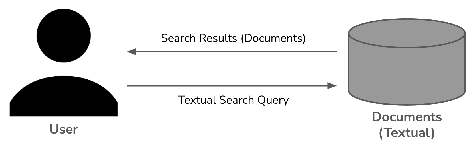
Searching for relevant training data is similar to any other search problem; see above. The only difference is that our query is an output from our LLM, rather than something that we input into a search bar. But, all of the same techniques for search can be applied to solving this problem. For a deep dive on this topic, check out the overview below. In this section, we will briefly cover the key concepts of search and how they can be applied to tracing training data.
The Basics of AI-Powered (Vector) Search

An introduction to modern search system and the role that LLMs play in making these systems more accurate.
Lexical search. For many years prior to the popularization of deep learning, most search engines were purely lexical, meaning that they rely on keyword (or n-gram) matches to find documents relevant to a query. To find these matches efficiently, we use a data structure called an inverted index. By counting matches between each query and document, as well as considering the uniqueness of each n-gram that is matched, we can derive a relevance score for each document. The most common algorithm for this is BM25, which is computed as shown below.

Although these details might seem complex, we can easily implement BM25-powered search via Python packages like rank_bm25 or bm25s. With these packages, we can build a search index over our data in Python and start running searches as shown in the code example below. As we can see, this functionality is easy to prototype and begin using without too much effort!
from transformers import AutoTokenizer
from rank_bm25 import BM25Okapi

tok = AutoTokenizer.from_pretrained(<your tokenizer>)

corpus = [
    "Here is a training example",
    "Here is another training example...",
]

tokenized_corpus = [doc.split(" ") for doc in corpus]

bm25 = BM25Okapi(tokenized_corpus)
Semantic search. Despite the power and efficiency of lexical search, this technique is still dependent upon keyword matching—semantic matches (i.e., different words with similar meaning) are not captured by this framework. If we want to handle semantic matches, we need to use some form of vector search; see below.

In vector search, we use an embedding model to produce and embedding for each document we want to search. Then, we store all of these embeddings in a vector database, which allows us to efficiently search for similar embeddings using algorithms like hierarchical navigable small worlds (HNSW). From here, we can simply embed our query and search for similar embeddings within the index, allowing us to find documents that are semantically similar to our query! This is exactly what is done by retrieval augmented generation (RAG) to retrieve relevant text chunks to add into the context of an LLM; see here for details.

The semantic search system outlined above uses bi-encoders, which produce separate embeddings—that are matched together via cosine similarity scores—for each document and query. However, we can also use cross-encoders, which take both the document and query as input and output a single similarity score. The difference between these two strategies is illustrated in the figure above. A variety of pretrained bi-encoders and cross-encoders are available in public repos and can be either finetuned or used out-of-the-box; see here for more details.
Modern search systems combine all of these techniques. A hybrid of both bi-encoders and (BM25) lexical search are first used to efficiently retrieve documents that are most relevant to our query. Then, we perform a fine-grained ranking of retrieved documents using a cross-encoder, bringing the most relevant documents to the top of the list; see below. All of these components can be finetuned over data collected as the search engine is used to improve their accuracy over time.

Applying search to debugging. Now that we understand the basics of search systems, we can also apply these ideas to debugging LLM outputs. However, there are two unique considerations for debugging LLM outputs that make this use case different from a standard search application:
LLM training datasets can be massive (tens of trillions of tokens), which can prohibit the use of some techniques.
Depending on the use case, the output of an LLM, as well as the documents over which the LLM is trained, can be very long.
If we are tracing a large dataset, using techniques like vector search—although not impossible—can be both time consuming and expensive. We have to first produce embeddings for our entire dataset, then store these embeddings in a vector database to make them searchable. This process requires a lot of setup (including the creation of large-scale data pipelines!), which makes the barrier to entry high.
Going further, the fact that our LLM’s outputs and training documents can be very long means that we need to approach this search problem differently. Instead of using the entire output as a search query, we need to consider shorter spans in this output and search for similar spans in the training data. Ideally, we want to develop a technique for tracing our training data that is:
Relatively simple to setup.
Efficient on large-scale datasets.
Able to operate on a (shorter) span level.
Infini-gram: Scaling Unbounded n-gram Language Models to a Trillion Tokens [1]
“Instead of pre-computing n-gram count tables (which would be very expensive), we develop an engine named infini-gram—powered by suffix arrays—that can compute ∞-gram (as well as n-gram with arbitrary n) probabilities with millisecond-level latency.” - from [1]
To understand how we can efficiently trace a massive dataset, we need to first understand the concept of an infini-gram [1]. Put simply, infini-grams are the generalization of n-grams to arbitrarily large values of N. As we will see, the data structure that we use to compute the probability of an infini-gram can also be used to (very efficiently) locate and count text spans of arbitrary length within a massive dataset. This property is very useful for model-focused curation and debugging!

What are n-gram LMs? An n-gram is simply an ordered set of N tokens (or words). Given a sequence of text, we can break it into n-grams as shown above, where we choose N = 3. If we break an entire dataset of text into n-grams, we can actually compute the probability of a given n-gram by simply counting the number of times that it occurs within the dataset; see below.

All of these counts are usually pre-computed and stored in a count table, allowing us to quickly lookup n-gram probabilities and evaluate the expression shown above. We can actually form a simple language model using n-gram probabilities! To predict the next token in a sequence using n-grams, we just:
Look at the last
N - 1tokens in the sequence.Get the probability of each possible n-gram given the prior
N - 1tokens.Sample the next token similarly to any other language model.
Limitations of n-grams. Practically speaking, n-gram LMs are not great at generating text—you will not be able to make a powerful chatbot by counting n-grams. Although this is true for any value of N, one of the key issues that limits the performance of n-gram LMs is the fact that n-gram count tables grow (almost) exponentially in size with respect to N. As a result, most n-gram LMs are limited to small values of N—e.g., N = 5 is a common setting—and have a low capacity for capturing meaningful, long-context language distributions; see below.

Additionally, n-gram LMs struggle with sparsity. Some n-grams may not appear in our data, forcing us to fall back to smaller n-grams to compute a probability—this concept is typically referred to as n-gram “backoff”. Forming a valid probability estimate when backing off to smaller n-grams is actually quite complicated.
Making n-grams relevant again. In [1], authors propose a variant of n-gram LMs—called infini-grams (or ∞-grams)—that mesh better with modern LLMs. Relative to standard n-grams, infini-grams make two key changes:
They are trained over a massive text dataset (trillions of tokens) like any other modern LLM, thus mitigating issues with sparsity.
The value of
Ncan be made arbitrarily large when computing the probability of an n-gram, which captures more meaningful distributions in the data.
What are ∞-grams? By making these changes, infini-grams solve the two biggest issues with n-gram LMs that we covered above. How does this work? Assume we have a textual sequence w. To compute the infini-gram of token i, we consider all tokens that precede token i in the sequence; see below.

On the left side of this equation, the infini-gram probability is conditioned on the entire prior context of the sequence, which is different from before. However, the right side of this equation exactly matches that of the n-gram probability! The key difference between n-grams and infini-grams lies in how we select the value of N.
For n-grams, N is a (fixed) hyperparameter. In contrast, infini-grams use a backoff procedure to dynamically select N. More specifically, we test the denominator of this expression with the largest possible N—all preceding tokens in the sequence—and continually decrease N by one until the denominator is non-zero; see below.
“We stop backing off as soon as the denominator becomes positive, upon which the numerator might still be zero… the effective n is equal to one plus the length of the prompt’s longest suffix that appears in the training data.” - from [1]
If we define w’as the subsequence of w up to (and including) token i - 1, then this backoff procedure is simply finding the longest suffix of w’ that exists in our dataset. From here, we use the value of N found via backoff to compute the infini-gram probability using the standard n-gram probability expression from before.
Computing ∞-gram probabilities. To compute infini-gram probabilities, we cannot just precompute counts and store them in a table like before. The value of N is unbounded and infini-grams are trained over LLM-scale datasets in [1]—the size of such a count table would be massive. Instead, we use a data structure called a suffix array to create an engine for efficiently computing infini-gram probabilities.

The concept of a suffix array is depicted above. Given a sequence of text w with length L, a suffix array is constructed by:
Extracting every suffix of this sequence (there are
Lof them).Sorting the suffixes lexicographically5.
Storing the original index (prior to sorting) of each sorted suffix within a list—this is the suffix array!
Consider w’ to be an arbitrary subarray of w running from token i to token j, where i < j. Any suffix that begins with w’ is stored consecutively in the suffix array due to the array being sorted lexicographically. Using this property, we can efficiently compute the count of w’ in w. We just find the index of the first and last suffix in the array for which w’ is a prefix, and the count of w’ in w is the difference between these two indices. If we can compute the count of w’, we can compute arbitrary infini-gram probabilities—this operation can be used to find N and compute both counts within the infini-gram probability expression!

∞-grams for LLMs. In the context of LLMs, our sequence w is the LLM’s entire tokenized training dataset, where document boundaries are marked with fixed separator token(s)6; see above. This sequence will be large—modern LLMs are trained on tens of trillion of tokens—but suffix arrays can handle data of this scale7.
“During inference, the entire infini-gram index can stay on-disk, which minimizes the compute resources needed (no GPU, and minimal CPU / RAM)… Our most optimized infini-gram engine can count a given n-gram with an average latency of less than 20 milliseconds. It can compute the probability and next-token distribution in 40 milliseconds for n-gram LMs, and in 200 milliseconds for the ∞-gram.” - from [1]
For example, the suffix array built over a 5T token dataset in [1] consumes ~35Tb of memory. Building this suffix array takes ~48 hours, and the entire suffix array can be stored on disk—even when computing infini-gram probabilties—after it is created. The resulting infini-gram engine can be used to compute probabilities for over two quadrillion unique n-grams. However, retrieving the count of a given n-gram on a dataset of this size still takes only ~20 milliseconds!
Using ∞-grams in practice. Fully grasping the ideas behind infini-grams will take some time. Luckily, the entire infini-gram project—similarly to any other project from Ai2—is fully open-source! There are plenty of open-source tools available for working with infini-grams in Python. See the project website for full details.
%pip install infini_gram
python -m infini_gram.indexing
    --data_dir <path to data>
    --save_dir <path to save index>
    --tokenizer llama  # also supports gpt2 and olmo
    --cpus <cpus available>
    --mem <memory available (in Gb)>
    --shards 1  # increase if N > 500B
    --add_metadata
    --ulimit 1048576
The tool that is most relevant to this overview is the inifini-gram Python package. Several open LLM training datasets have already been pre-indexed within this package, but we can also use the package to build an infini-gram index over our custom dataset using the command above. Once the index is available, we can use the infini-gram Python package to efficiently run a variety of different search and counting operations; see below for examples and here for more details.
from infini_gram.engine import InfiniGramEngine
from transformers import AutoTokenizer

# instantiate tokenizer (must match tokenizer used for indexing)
tokenizer = AutoTokenizer.from_pretrained(
    "meta-llama/Llama-2-7b-hf",
    add_bos_token=False,
    add_eos_token=False,
)

# connect to infini-gram engine
engine = InfiniGramEngine(
    index_dir=<path to index>,
    eos_token_id=tokenizer.eos_token_id,
)

# sample n-gram / sequence
inp = "This is my sample n-gram sequence."
inp_ids = tokenizer.encode(inp)

# find matching n-grams in dataset
result = engine.find(input_ids=input_ids)

# n-gram count
result = engine.count(input_ids=inp_ids)

# n-gram probability
result = engine.prob(
    prompt_ids=inp_ids[:-1],
    cont_id=inp_ids[-1],
)

# next token distribution
result = engine.ntd(prompt_ids=inp_ids)

# infini-gram probability
result = engine.infgram_prob(
    prompt_ids=inp_ids[:-1],
    cont_id=inp_ids[-1],
)
OLMoTrace: Tracing Language Model Outputs Back to Trillions of Training Tokens [2]

OLMoTrace [2] pioneers a novel approach for efficiently attributing the output of an LLM to examples within its training data. This approach is deployed within the Ai2 playground (shown above) and can perform a trace to retrieve training documents that are relevant to an LLM’s output in seconds. Given that LLMs are trained over massive datasets, we might wonder how such a real-time trace would be possible. Luckily, we have already learned the answer: infini-grams!
“The purpose of OLMOTRACE is to give users a tool to explore where LMs may have learned to generate certain word sequences, focusing on verbatim matching as the most direct connection between LM outputs and the training data.” - from [2]
Tracing strategy. The key idea behind OLMoTrace is to find examples of long and unique token sequences that are present both in the model’s output and its training dataset. Given a prompt and LLM response as input, OLMoTrace will return the following:
A set of notable textual spans found in the LLM’s response.
A list of the most relevant document spans from the LLM’s training data associated with each response span.
Unlike vector search, these matches between the model’s output and training data must be verbatim. Exact token matches can be quickly identified with a suffix array, as discussed in the last section. However, ensuring that the best possible matching documents are identified and returned requires a four-step algorithm that is built on top of the standard infini-gram functionality.
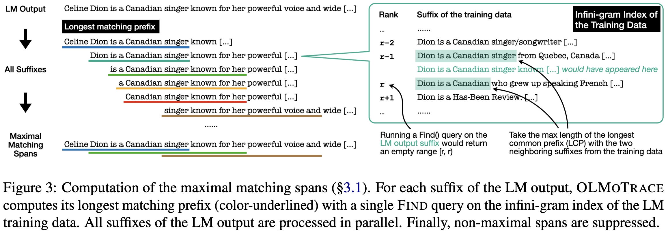
(Step 1) Maximal Matching Spans. After tokenizing the LLM’s response, we find all text spans in this response that satisfy three properties:
Existence: the span has an exact match in the training data.
Maximality: the span is not a sub-span of another matching span.
Self-contained: the span is not incomplete; e.g., beginning or ending with incomplete words or containing punctuation in the middle of the span.
These properties are illustrated within the figure below. Here, we see that there are three matching spans. However, all spans except for one—outlined in green—are removed due to either not being i) maximal or ii) self-contained.

Computing maximal spans naively is inefficient, but authors in [2] propose a more efficient algorithm that relies upon the find operation in the infini-gram index. Given a sequence of tokens as input, the find operation returns:
The count of matching spans in the index.
A range of segments8 that can be used to look up matching data spans.
However, if the returned count is zero—indicating that our data has no exact matches for this sequence—the find operation will still return an (empty) segment range. Because the suffix array is sorted lexicographically, the index of this range corresponds to the longest matching prefix of the sequence in our dataset.
# run find operation with infini-gram engine
result = engine.find(input_ids=inp_ids)

"""
### .find() output example (match):
    {
        'cnt': 10,
        'segment_by_shard': [(13693395, 13693405)],
    }

### .find() output example (no match):
    {
        'cnt': 0,
        'segment_by_shard': [(85267640, 85267640)],
    }
"""

# lookup training documents from .find()
rank_start, rank_end = result['segment_by_shard'][0]
ranks = [r for r in range(rank_start, rank_end)]
for r in ranks:
    docs = engine.get_doc_by_rank(
        s=0,  # assumes suffix array has a single shard
        rank=r,
        max_disp_len=len(inp_ids) * 5,  # size of doc chunk
    )
    doc_text = [tokenizer.decode(d['token_ids']) for d in docs]
    print(f'Number of documents: {len(docs)}')
    print(f'Matching document: {doc_text[0]}')
This property of the find operation is leveraged in [2] to create an efficient algorithm for span matching. As shown in the figure below, this algorithm operates by running a single find operation for every suffix of the input sequence, yielding the longest matching prefix for each suffix. Once all of these matching spans have been identified, we can make another pass through this list to remove any matching spans that are not maximal or self-contained.
(Step 2) Span Filtering. If our list of maximal spans computed as described above is long, we need some strategy to identify the most useful and relevant of these spans. To do this, authors in [2] score spans according to their span unigram probability (lower is better)—or the product of unigram probabilities for each token in the span. The unigram probability of a given token, which is usually precomputed for all tokens and stored in a cache, can be computed as shown below.

In [2], authors sort spans by their span unigram probability and keep only the first K spans in this list, where K = ceil(0.05 x L) for a sequence of length L.
(Step 3-4) Merge Spans and Get Documents. To avoid clutter, overlapping spans are merged together in OLMoTrace. Documents for each of these final spans are retrieved. But, the number of documents associated with each span can be large, so we must sub-select documents; e.g., authors in [2] retain ten documents per span. To find the most relevant documents, we can rank them according to the BM25 score between the LLM’s output and the retrieved document.
“To prioritize showing the most relevant documents, in the document panel we rank all documents by a BM25 score in descending order. The per-document BM25 score is computed by treating the collection of retrieved documents as a corpus, and the concatenation of user prompt and LM response as the query.” - from [2]

Example implementation. The inference pipeline for OLMoTrace is shown in the figure above. To better understand how this works, let’s (quickly) implement the core functionality using the infini-gram package in Python. To build an infini-gram index, we need to put all of our LLM’s training data into a single directory. The infini-gram package expects the data to be formatted as one or more .jsonl files, where each file contains text and metadata fields; see below. Each line of the .jsonl file corresponds to a single document in our training dataset.
{
    'text': 'This is a training sequence for our LLM...',
    'metadata': {
        'source': <url>,
        'category': 'general',
        'year': 2025,
        ...
    },
}
Once our data has been formatted as such, we can build the infini-gram index as outlined before. Additionally, OLMoTrace requires us to pre-compute unigram probabilities for all tokens. Both of these steps are implemented below. This code assumes that we use the Llama 2 tokenizer to perform tracing and that we only require a single shard for our infini-gram index. The underlying tokenizer can be modified, and support for multiple shards in the index may be required when working with very large datasets (i.e., more than 500B tokens).
| import os | |
| import json | |
| from collections import Counter | |
| import tempfile | |
| from transformers import AutoTokenizer | |
| # load tokenizer / data | |
| enc = AutoTokenizer.from_pretrained("meta-llama/Llama-2-7b-hf", add_bos_token=False, add_eos_token=False) | |
| data_rows = [{'text': 'here is some training data'}, ...] | |
| # compute / save unigram probabilities | |
| all_toks = [] | |
| for x in data_rows: | |
| all_toks.extend(enc.encode(x['text'])) | |
| total_toks = len(all_toks) | |
| tok_count = Counter(all_toks) | |
| unigram_probs = {} | |
| for tid in tok_count: | |
| cnt = tok_count[tid] | |
| unigram_probs[tid] = cnt / total_toks | |
| with open(<save path>, 'w') as json_file: | |
| json.dump(unigram_probs, json_file, indent=4) | |
| # build infinigram index | |
| data_dir = <path to data> | |
| save_dir = <save index here> | |
| temp_dir = tempfile.TemporaryDirectory() | |
| command = ( | |
| f"python -m infini_gram.indexing --data_dir {data_dir} " | |
| f"--temp_dir {temp_dir.name} --save_dir {save_dir} " | |
| f"--tokenizer llama --cpus 12 --mem 64 --shards 1 " | |
| f"--add_metadata --ulimit 100000 " | |
| ) | |
| print(command) | |
| os.system(command) | |
| temp_dir.cleanup() |
Now that the infini-gram index has been built, we can trace a sequence of text over our training dataset—following the algorithm proposed by OLMoTrace in [2]—as shown in the code below. This code returns both a set of spans and their associated documents with metadata from the training corpus.
| import ast | |
| import math | |
| import random | |
| from infini_gram.engine import InfiniGramEngine | |
| from transformers import AutoTokenizer | |
| def compute_longest_prefix(query, doc): | |
| """helper function for computing longest prefix of query that exists | |
| within a document""" | |
| def shared_prefix_length(list1, list2): | |
| prefix_length = 0 | |
| for elem1, elem2 in zip(list1, list2): | |
| if elem1 == elem2: | |
| prefix_length += 1 | |
| else: | |
| break | |
| return prefix_length | |
| first_id = query[0] | |
| start_idx = [index for index, value in enumerate(doc) if value == first_id] | |
| longest_prefix = 0 | |
| for si in start_idx: | |
| longest_prefix = max( | |
| longest_prefix, | |
| shared_prefix_length(query, doc[si:]), | |
| ) | |
| return longest_prefix | |
| # setup | |
| enc = AutoTokenizer.from_pretrained("meta-llama/Llama-2-7b-hf", add_bos_token=False, add_eos_token=False) | |
| engine = InfiniGramEngine(index_dir=<path to index>, eos_token_id=enc.eos_token_id) | |
| unigram_probs = {1: 0.5, 2: 0.5} # load pre-computed probabilities | |
| # LLM output / query to search | |
| generation = 'Here is the output of the LLM that we want to search for in our data.' | |
| gen_ids = enc.encode(generation) | |
| """ | |
| Step One: find maximal matching spans | |
| """ | |
| L = len(gen_ids) | |
| max_doc_toks = len(gen_ids) * 2 # size of spans to retrieve in documents | |
| # find longest prefix match for every suffix in the query | |
| spans = [] | |
| for start in range(len(gen_ids) - 1): | |
| _suffix = gen_ids[start:] | |
| _suff_res = engine.find(input_ids=_suffix) | |
| # if no match, get the longest matching prefix using find result | |
| if _suff_res['cnt'] == 0: | |
| _shards = _suff_res['segment_by_shard'] | |
| assert len(_shards) == 1 # assume only one shard | |
| _doc_ids = engine.get_doc_by_rank( | |
| s=0, # assume only one shard | |
| rank=_shards[0][0], | |
| max_disp_len=max_doc_toks, | |
| )['token_ids'] | |
| matched_toks = compute_longest_prefix(_suffix, _doc_ids) # get longest matching prefix | |
| elif _suff_res['cnt'] > 0: | |
| matched_toks = len(_suffix) | |
| spans.append((start, start + matched_toks)) | |
| # remove partial and non-self-contained spans | |
| full_spans = [] | |
| for start, end in spans: | |
| span_ids = gen_ids[start: end] | |
| span_text = enc.decode(span_ids) | |
| # check for internal punctuation | |
| has_internal_punc = False | |
| punc_chars = "!.?\n" | |
| for ch in span_text[:-1]: | |
| if ch in punc_chars: | |
| has_internal_punc = True | |
| break | |
| if has_internal_punc: | |
| continue | |
| # check if first token is a continuation of a word | |
| first_tok_id = span_ids[0] | |
| first_tok = enc.convert_ids_to_tokens(first_tok_id) | |
| if first_tok[0] != '▁': # assumes Llama 2 token format | |
| continue | |
| # no sub-token follows the last token | |
| if end < len(gen_ids) and tokenizer.convert_ids_to_tokens(gen_ids[end])[0] != "▁": | |
| continue | |
| full_spans.append((start, end, span_ids, span_text)) | |
| # remove non-maximal spans | |
| maximal_spans = [] | |
| max_end_pos = -1 | |
| full_spans = sorted(full_spans) | |
| for start, end, ids, text in full_spans: | |
| if end > max_end_pos: | |
| maximal_spans.append((start, end, ids, text)) | |
| max_end_pos = end | |
| """ | |
| Step Two: filter to keep long / unique spans | |
| """ | |
| K = math.ceil(0.05 * L) | |
| assert K > 0 | |
| filt_spans = [] | |
| for start, end, ids, text in maximal_spans: | |
| span_uni_prob = [unigram_probs.get(_id) for _id in ids] | |
| span_uni_prob = math.prod(span_uni_prob) | |
| filt_spans.append((start, end, ids, text, span_uni_prob)) | |
| filt_spans = sorted(filt_spans, key=lambda x: x[-1]) | |
| filt_spans = filt_spans[:K] | |
| filt_spans = sorted(filt_spans) # sort based on start position again | |
| """ | |
| Step Three: retrieve Enclosing Docs | |
| """ | |
| docs_per_span = 10 | |
| span_to_docs = defaultdict(list) | |
| for i, (start, end, ids, text, uni_prob) in enumerate(filt_spans): | |
| # run retrieval in infinigram index to get documents | |
| span_res = engine.find(input_ids=ids) | |
| assert span_res['cnt'] > 0 | |
| assert len(span_res['segment_by_shard']) == 1 # assume only one shard | |
| rank_start, rank_end = span_res['segment_by_shard'][0] | |
| ranks = [r for r in range(rank_start, rank_end)] | |
| if len(ranks) > docs_per_span: | |
| # retrieve fixed number of documents for each span | |
| ranks = sorted(random.sample(ranks, docs_per_span)) | |
| # NOTE: we can instead rank documents by BM25 score here! | |
| for r in ranks: | |
| _doc = engine.get_doc_by_rank( | |
| s=0, | |
| rank=r, | |
| max_disp_len=max_doc_toks, | |
| ) | |
| _doc_meta = ast.literal_eval(_doc['metadata'])['metadata'] | |
| _doc_text = enc.decode(_doc['token_ids']) | |
| _doc_data = { | |
| "text": _doc_text, | |
| **_doc_meta | |
| } | |
| span_to_docs[i].append(_doc_data) | |
| """ | |
| Step Four: merge overlapping spans | |
| """ | |
| # get indices of spans to merge together | |
| merged_spans = [[0]] | |
| curr_idx = 0 | |
| curr_start = filt_spans[0][0] | |
| curr_end = filt_spans[0][1] | |
| for i, next_span in enumerate(filt_spans[1:]): | |
| start = next_span[0] | |
| end = next_span[1] | |
| if start < curr_end: | |
| curr_end = max(curr_end, end) | |
| merged_spans[curr_idx].append(i + 1) | |
| else: | |
| curr_start, curr_end = start, end | |
| curr_idx += 1 | |
| merged_spans.append([i + 1]) | |
| assert len(merged_spans) == curr_idx + 1 | |
| # merge spans into a final set | |
| final_spans = [] | |
| for ms in merged_spans: | |
| all_docs = [] | |
| docs_per_merged_span = math.ceil(docs_per_span / float(len(ms))) # subsample docs for spans being merged | |
| for i in ms: | |
| # take top docs from each span being merged | |
| all_docs.extend(span_to_docs[i][:docs_per_merged_span]) | |
| _spans = [filt_spans[i] for i in ms] | |
| start = min([x[0] for x in _spans]) | |
| end = max([x[1] for x in _spans]) | |
| text = enc.decode(gen_ids[start: end]) | |
| final_spans.append({ | |
| "start": start, | |
| "end": end, | |
| "text": text, | |
| "docs": all_docs, | |
| }) | |
| """ | |
| Step Five: observe tracing results | |
| """ | |
| docs_to_print = 5 | |
| print(f'Query Text: {enc.decode(gen_ids)}') | |
| for i, sp in enumerate(final_spans): | |
| print("\n" + "="*20 + f" SPAN {i + 1} / {len(final_spans)} " + "="*20) | |
| print(f"Span Text: {sp['text']}\n") | |
| for j, doc in enumerate(sp['docs']): | |
| print("-"*10 + f" Document {j + 1} / {len(sp['docs'])} " + "-"*10) | |
| for k in ['text', 'movie_id', 'src_lang', 'start_frame', 'end_frame']: | |
| if k == 'text': | |
| v = doc[k].replace('\n', ' ') | |
| else: | |
| v = doc[k] | |
| print(f"- {k} --> {v}") |
As we can see, the core functionality of OLMoTrace is not that complicated—most of the complex code is already abstracted away by the infini-gram package! For those who are interested, I would highly recommend testing out this code on your own model and data to get a feel for the types of results it can return!

Applications of OLMoTrace. OLMoTrace specializes in finding long and unique spans that exactly match between an LLM’s output and its training data. Exact matches are a useful proxy for finding training data that may contribute to a certain output from our LLM. In [2], a variety of different use cases are considered:
Fact checking: compare factual statements made by the LLM to similar factual statements within its training data.
Creative expressions: check if “creative” outputs from the LLM are actually creative, or just directly copied from training data.
Reasoning capabilities: check if the LLM copies the reasoning process used to solve verifiable problems (e.g., math) from its training data.
In each of these cases, we can learn something new about our LLM by tracing its output to find regions of the training data with a notable, verbatim match.
Reasoning Models and Future Research
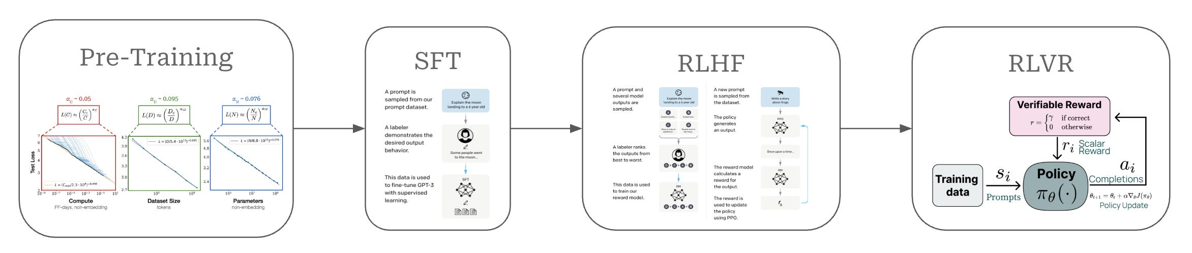
Extension to reasoning models. As shown above, LLMs are usually trained in several phases, each of which have unique styles of data:
Supervised Finetuning (SFT): trains the LLM using concrete examples of prompt-response pairs that the LLM should replicate.
Reinforcement Learning from Human Feedback (RLHF): trains the model using preference pairs (i.e., a single prompt with two responses, where one of the two responses is identified as better than the other).
Reinforcement Learning from Verifiable Rewards (RLVR): uses pure RL to reward the model for correctly solving verifiable problems as determined by a rule-based (usually deterministic) verification function.
Despite these unique data formats, we can apply OLMoTrace to each stage of training with minimal changes! We can easily build an infini-gram index over supervised examples and preference pairs (though we may want to treat the positive and negative completions in the preference pair differently). For RLVR, however, we may need to think more deeply about how the data should be traced.
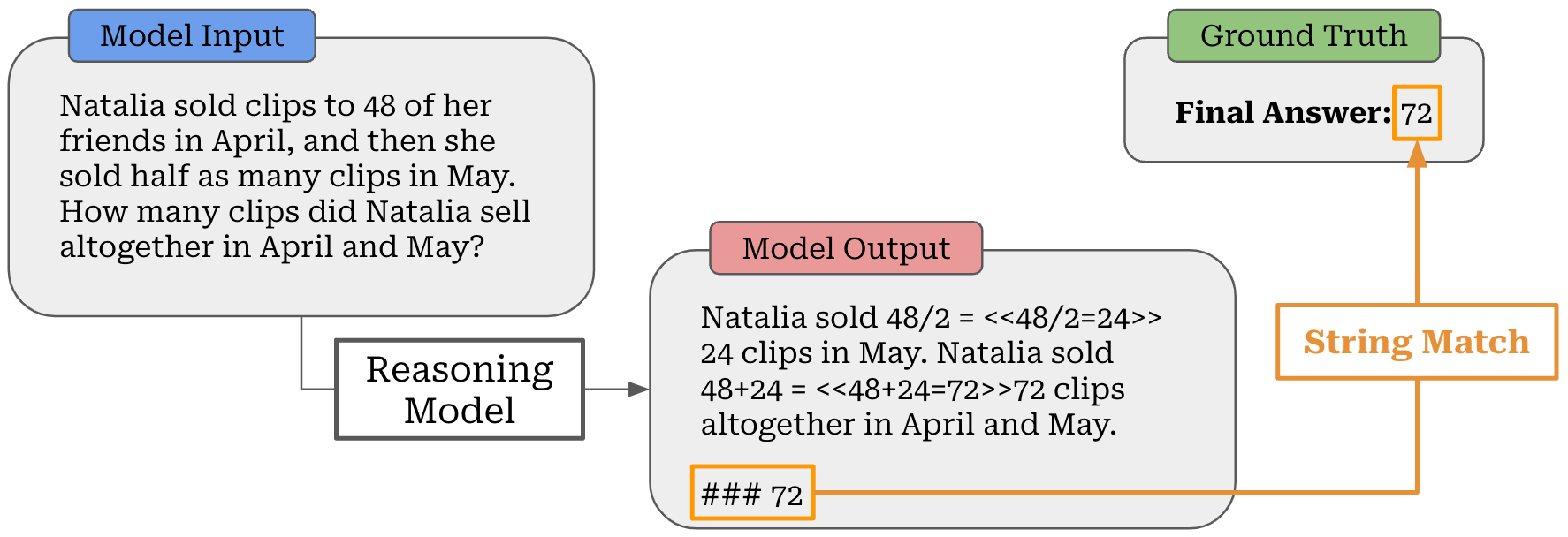
When training an LLM with RLVR, we have a dataset of problems with verifiable solutions; e.g., a math problem with a known solution or a coding problem with test cases. We can easily check whether the LLM solves such problems correctly (e.g., by string matching or something slightly more robust); see above. Then, the model learns how to solve these problems on its own via a self-evolution process powered by large-scale RL training, as demonstrated by DeepSeek-R1 [7].
“We explore the potential of LLMs to develop reasoning capabilities without any supervised data, focusing on their self-evolution through a pure reinforcement learning process.” - from [7]
During RL training, we see in [7] that LLMs learn to output complex chains of thought—sometimes thousands of tokens in length!—to improve their reasoning capabilities. If we want to index these reasoning traces, however, we run into an interesting problem. Namely, the reasoning traces are not actually part of our training data—they are generated by the LLM during the RL training process.

Similarly, the LLM generates completions that are ranked by a reward model and used for policy updates during RLHF; see here for further explanation. If we want to capture patterns learned during RL training—including both RLHF and RLVR—we have to keep track of the completions generated by our LLM during training. Given access to these completions, we can index them like any other training data, add them to an infini-gram index, and trace them using OLMoTrace.
Related (and future) research. Despite the utility of OLMoTrace, exact matches do NOT guarantee causality—there are many reasons an LLM may have generated an output. Just because we find training data that is similar to an output from our LLM does not mean that this data is guaranteed to have caused this output.
Attempting to provide deeper insight into the outputs of an LLM, several parallel veins of research are investigating alternative strategies for explainability. For example, many papers have been recently published on the topic of teaching LLMs how to cite sources when generating output [8, 9, 10]; see below.

Such an ability to cite sources can be incorporated into the LLM’s standard training process—e.g., pretraining [8] or RLHF [9]—such that the model learns when and how to provide evidence for its answers. However, there is still no guarantee that these citations truly explain how an output was generated.
The field of mechanistic interpretability seeks to study the internals of neural networks to gain an understanding of why they produce the outputs that they do. Although deep neural networks are typically portrayed as block boxes, we can discover many repeated circuits and features in these networks when studied at a microscopic level (i.e., small sets of weights). For example, vision networks tend to have dedicated units for detecting curves, edges and much more.

The topic of mechanistic interpretability was largely popularized by Anthropic. In a recent report, researchers performed a large-scale study of features in Claude Sonnet using dictionary learning. As shown above, this study discovered millions of features for advanced concepts, such as people, places, bugs in code and more.
“We have identified how millions of concepts are represented inside Claude Sonnet, one of our deployed large language models. This is the first ever detailed look inside a modern, production-grade large language model.” - from [11]
Additionally, authors analyze the “distance” between features and find some interesting properties; e.g., the Golden Gate Bridge feature is close to that of Alcatraz. Such research, though nascent, is arguably the most promising avenue for truly understanding why and how LLMs produce certain outputs.
Conclusions
As we have learned, optimizing our training dataset is one of the most impactful and important aspects of the LLM training process. To effectively curate and debug our data, we should begin by looking at the data itself—not by training models! First, we should manually inspect our data and develop an understanding of its various properties, patterns and quirks. To scale the manual inspection process, we can rely upon both heuristics (when possible) and machine learning models; e.g., fastText or LLM judges. This data-focused curation process focuses upon fixing issues and improving data quality before training any LLMs!
“One pattern I noticed is that great AI researchers are willing to manually inspect lots of data. And more than that, they build infrastructure that allows them to manually inspect data quickly. Though not glamorous, manually examining data gives valuable intuitions about the problem.” - Jason Wei
Once we start training LLMs, we can use the LLM’s outputs to find issues in our data. More specifically, we can:
Identify problematic LLM outputs via our evaluation framework.
Trace these outputs to corresponding regions of the training data.
Although we can use standard search techniques—like lexical or vector search—for tracing data, there are specialized tracing techniques that have been specifically developed for LLMs like OLMoTrace [2]. These techniques are easy (and quick) to setup, highly informative and can be scaled to arbitrarily large datasets, making them a very practical choice for debugging LLM training datasets.
New to the newsletter?
Hi! I’m Cameron R. Wolfe, Deep Learning Ph.D. and Senior Research Scientist at Netflix. This is the Deep (Learning) Focus newsletter, where I help readers better understand important topics in AI research. If you like the newsletter, please subscribe, share it, or follow me on X and LinkedIn!
Bibliography
[1] Liu, Jiacheng, et al. "Infini-gram: Scaling unbounded n-gram language models to a trillion tokens." arXiv preprint arXiv:2401.17377 (2024).
[2] Liu, Jiacheng, et al. "OLMoTrace: Tracing Language Model Outputs Back to Trillions of Training Tokens." arXiv preprint arXiv:2504.07096 (2025).
[3] Touvron, Hugo, et al. "Llama 2: Open foundation and fine-tuned chat models." arXiv preprint arXiv:2307.09288 (2023).
[4] Kaplan, Jared, et al. "Scaling laws for neural language models." arXiv preprint arXiv:2001.08361 (2020).
[5] Ouyang, Long, et al. "Training language models to follow instructions with human feedback." Advances in neural information processing systems 35 (2022): 27730-27744.
[6] Lambert, Nathan, et al. "T\" ulu 3: Pushing frontiers in open language model post-training." arXiv preprint arXiv:2411.15124 (2024).
[7] Guo, Daya, et al. "Deepseek-r1: Incentivizing reasoning capability in llms via reinforcement learning." arXiv preprint arXiv:2501.12948 (2025).
[8] Khalifa, Muhammad, et al. "Source-aware training enables knowledge attribution in language models." arXiv preprint arXiv:2404.01019 (2024).
[9] Glaese, Amelia, et al. "Improving alignment of dialogue agents via targeted human judgements, 2022." URL https://storage. googleapis. com/deepmind-media/DeepMind. com/Authors-Notes/sparrow/sparrow-final. pdf (2022).
[10] Huang, Chengyu, et al. "Training language models to generate text with citations via fine-grained rewards." arXiv preprint arXiv:2402.04315 (2024).
[11] Anthropic. “Mapping the Mind of a Large Language Model” https://www.anthropic.com/research/mapping-mind-language-model (2025).
[12] Liu, Yang, et al. "G-eval: NLG evaluation using gpt-4 with better human alignment." arXiv preprint arXiv:2303.16634 (2023).
[13] Meta. “The Llama 4 herd: The beginning of a new era of natively multimodal AI innovation”https://ai.meta.com/blog/llama-4-multimodal-intelligence/(2025).
The papers that generate the largest interest tend to fall into this category; e.g., recent examples include GRPO, diffusion LLMs, and RLVR.
Specifically, Llama 3 was post-trained using only SFT and DPO, while Llama 4 uses a more sophisticated pipeline of SFT, online RL, and lightweight DPO; see here.
The rule of thumb for what constitutes “enough” manual data inspection is that it’s more than you want it to be. Seriously, spend more time manually inspecting your data. You won’t regret it!
For example, Llama 3 has a multi-stage pretraining process where select data sources (e.g., reasoning datasets) are emphasized more heavily in later stages to improve the model’s capabilities in certain domains; see here.
Lexicographical ordering is a generalization of alphabetical ordering to support characters that go beyond the alphabet (e.g., numbers and symbols).
In [1], authors use the \xff\xff token as a separator between documents.
Assume that our dataset contains T tokens and that the vocabulary size of our tokenizer is ~64K, meaning that each token ID can be represented with two bytes. The list of token IDs for this dataset consumes 2T bytes. The suffix array is a list of T indices that point to positions in the token array, where each index is represented with log(2T)/8 bytes. If 2B < T < 500B, indices can be stored using 5 bytes, meaning that the combined size of the token and suffix arrays is just 7T bytes!
These segments are just integers corresponding to the position of a matching span within the full token array.
https://nandigamharikrishna.substack.com/p/why-llms-hallucinate-every-type-and?r=8op1j&utm_campaign=post&utm_medium=web
Hi cameron, Great writing, on this A Guide for Debugging LLM Training Data topic, just started on substacl to write AI focus writing, do review https://deeprightai.substack.com/?utm_campaign=pub&utm_medium=web my writing, and suggest more improvements?