nanoMoE: Mixture-of-Experts (MoE) LLMs from Scratch in PyTorch

An introductory, simple, and functional implementation of MoE LLM pretraining...

Research on large language models (LLMs) has progressed at a shocking pace over the last several years. However, the architecture upon which most LLMs are based—the decoder-only transformer—has remained fixed despite the chaotic and rapid advancements in this field. More recently, we are starting to see a new¹ architecture, called a Mixture-of-Experts (MoE), being adopted in top research labs. For example, GPT-4 is rumored to be MoE-based, as well as the recently-proposed—and very popular—DeepSeek-v3 and R1 models; see below.

“To further push the boundaries of open-source model capabilities, we scale up our models and introduce DeepSeek-V3, a large Mixture-of-Experts (MoE) model with 671B parameters, of which 37B are activated for each token.” - from [8]

MoE-based LLMs use a modified version of the decoder-only transformer that has become popular due to an ability to make the training and usage of large models more efficient. MoE-based LLMs are very large in terms of their number of total parameters. However, only a subset of these parameters—selected dynamically during inference—are used when computing the model’s output. The sparsity of MoEs drastically reduces the cost of very large and powerful LLMs.

Given that many frontier LLMs are starting to use MoE-based architectures, developing an in-depth understanding of MoEs is important. In this post, we will take a step in this direction by building (and pretraining) a mid-sized MoE model—called nanoMoE—from scratch in PyTorch. All of the code for nanoMoE is available in the repository below, which is a fork of Andrej Karpathy’s nanoGPT library that has been expanded to support MoE pretraining. To understand how nanoMoE works, we will start by outlining necessary background information. Then, we will build each component of nanoMoE from the ground up, eventually culminating in a (successful) pretraining run for the model.

Basics of Decoder-Only Transformers

Decoder-Only Transformers: The Workhorse of Generative LLMs

In order to understand MoE-based LLMs, we first need to understand the standard architecture upon which most LLMs are based—the decoder-only transformer architecture. This architecture is a modified version of the encoder-decoder transformer architecture [1] that was popularized by GPT. Although we have studied this architecture deeply in prior posts (see above), we will go over it again here, as this knowledge is essential to the rest of the post. While explaining the architecture, we will rely on Andrej Karpathy’s nanoGPT—a minimal and functional implementation of decoder-only transformers—as a reference.

(from [1])

Original architecture. The transformer, originally proposed for solving machine translation tasks in [1], has both an encoder and a decoder module; see above. We will not focus on the full (encoder-decoder) transformer here. However, a detailed (and widely cited) overview of this architecture can be found here.

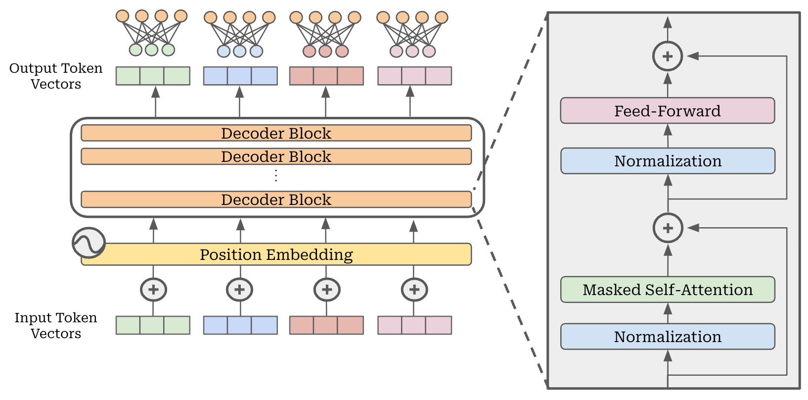
The decoder-only transformer, which is more commonly-used for modern LLMs, simply removes the encoder from this architecture and uses only the decoder², as indicated by the name. Practically, this means that every layer of the decoder-only transformer architecture contains the following:

1. A masked self-attention layer.

2. A feed-forward layer.

To form the full decoder-only transformer architecture, we just stack L of these layers, which are identical in structure but have independent weights, on top of each other. A depiction of this structure is provided in the figure below.

The decoder-only transformer architecture

Let’s now discuss each component of the architecture in isolation to gain a better understanding. We will start with the input structure for the model, followed by the components of each layer (i.e., self-attention and feed-forward layers) and how they are combined to form the full model architecture.

From Text to Tokens

As most of us probably know, the input to an LLM is just a sequence of text (i.e., the prompt). However, the input that we see in the figure above is not a sequence of text! Rather, the model’s input is a list of token vectors. If we are passing text to the model as input, how do we produce these vectors from our textual input?

Converting raw text into a sequence of tokens

Tokenization. The first step of constructing the input for an LLM is breaking the raw textual input—a sequence of characters—into discrete tokens. This process, called tokenization, is handled by the model’s tokenizer. There are many kinds of tokenizers, but Byte-Pair Encoding (BPE) tokenizers [2] are the most common; see here for more details. These tokenizers take a sequence of raw text as input and break this text into a sequence of discrete tokens as shown in the figure above.

This file contains bidirectional Unicode text that may be interpreted or compiled differently than what appears below. To review, open the file in an editor that reveals hidden Unicode characters. Learn more about bidirectional Unicode characters

Show hidden characters

	import torch
	from transformers import AutoTokenizer
	# load the llama-3.2 tokenizer
	tokenizer = AutoTokenizer.from_pretrained('meta-llama/Llama-3.1-8B')
	# raw text
	text = "This raw text will be tokenized"
	# create tokens using tokenizer
	tokens = tokenizer.tokenize(text)
	token_ids = tokenizer.convert_tokens_to_ids(tokens)
	# token_ids = tokenizer.encode(text) # directly create token ids
	# view the results
	print("Original Text:", text)
	print("Tokens:", tokens)
	print("Token IDs:", token_ids)
	# create token embedding layer
	VOCABULARY_SIZE: int = 128000
	EMBEDDING_DIM: int = 768
	token_embedding_layer = torch.nn.Embedding(
	num_embeddings=VOCABULARY_SIZE,
	embedding_dim=EMBEDDING_DIM,
	)
	# get token embeddings (IDs must be passed as a tensor, not a list)
	token_emb = token_embedding_layer(torch.tensor(token_ids))
	print(f'Token Embeddings Shape: {token_emb.shape}')

view raw tokenizer_example.py hosted with ❤ by GitHub

Packages for training and interacting with LLMs (e.g., HuggingFace or torchtune) provide interfaces for interacting with tokenizers. Additionally, OpenAI has released the tiktoken package for interacting with GPT tokenizers. The code snippet above tokenizes a textual sequence as follows:

• Raw Text: This raw text will be tokenized

• Tokenized Text: ['This', 'Ġraw', 'Ġtext', 'Ġwill', 'Ġbe', 'Ġtoken', 'ized']

Here, the Ġ character indicates that a token immediately follows a whitespace. Such special characters are tokenizer-dependent. For example, many tokenizers instead use a # character to indicate the continuation of a word, which would yield['token', '#ized'] for the final two tokens in the above sequence.

Vocabulary. Each LLM is trained with a specific tokenizer, though a single tokenizer may be used for several different LLMs. The set of tokens that can be produced by a given tokenizer is also fixed. As such, an LLM has a fixed set of tokens that it understands (i.e., those produced by the tokenizer) and is trained on. This fixed set of tokens is colloquially referred to as the LLM’s “vocabulary”; see below. Vocabulary sizes change between models and depend on several factors (e.g., multilingual models tend to have larger vocabularies), but vocabulary sizes of 64K to 256K total tokens are relatively common for recent LLMs.

Token vocabulary (and vectors) for an LLM

Token IDs and Embeddings. Each token in the LLM’s vocabulary is associated with a unique integer ID. For example, the prior code yields this sequence of IDs when tokenizing our text: [2028, 7257, 1495, 690, 387, 4037, 1534]. Each of these IDs is associated with a vector, known as a token embedding, in an embedding layer. An embedding layer is just a large matrix that stores many rows of vector embeddings. To retrieve the embedding for a token, we just lookup the corresponding row—given by the token ID—in the embedding layer; see above.

Input matrix of token embeddings (or vectors)

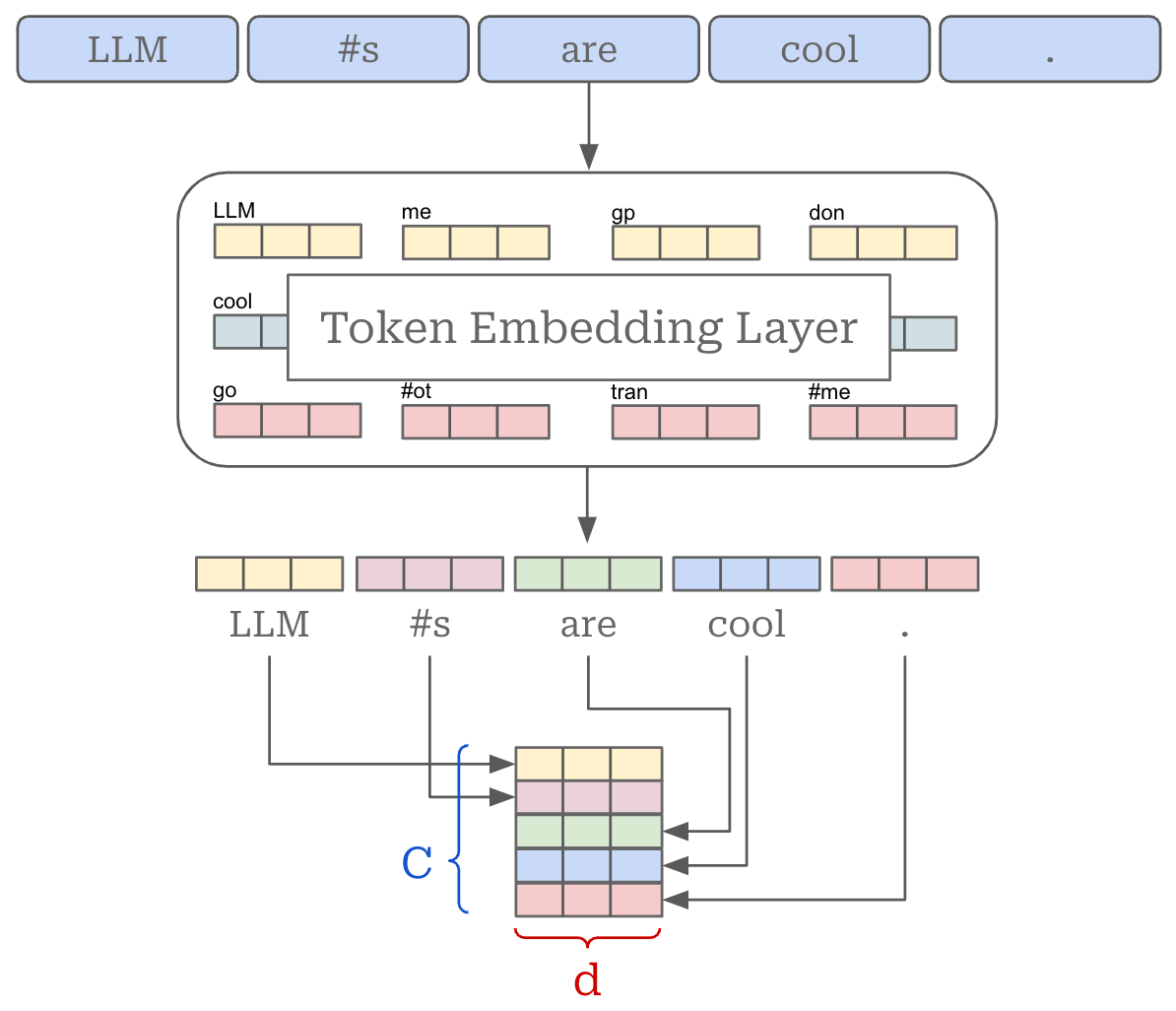
We now have a list of token embeddings. We can stack these embeddings into a matrix to form the actual input that is ingested by the transformer architecture; see above. In PyTorch, the creation of this matrix is handled automatically by the tokenizer and embedding layer, as shown in the prior code.

The token embedding matrix is of size [C, d], where C is the number of tokens in our input and d is the dimension of token embeddings that is adopted by the LLM. We usually have a batch of B input sequences instead of a single input sequence, forming an input matrix of size [B, C, d]. The dimension d impacts the sizes of all layers or activations within the transformer, which makes d an important hyperparameter choice. Prior to passing this matrix to the transformer as input, we also add a positional embedding to each token in the input³, which communicates the position of each token within its sequence to the transformer.

(Masked and Multi-Headed) Self-Attention

Now, we are ready to pass our input—a token embedding matrix—to the decoder-only transformer to begin processing. As previously outlined, the transformer contains repeated blocks with self-attention and a feed-forward transformation, each followed by normalization operations. Let’s look at self-attention first.

(from [1])

What is self-attention? Put simply, self-attention transforms the representation of each token in a sequence based upon its relationship to other tokens in the sequence. Intuitively, self-attention bases the representation of each token on the other tokens in the sequence (including itself) that are most relevant to that token. In other words, we learn which tokens to “pay attention” to when trying to understand the meaning of a token in our sequence. For example, we see above that the representation for the word making is heavily influenced by the words more and difficult, which help to convey the overall meaning of the sentence.

“An attention function [maps] a query and a set of key-value pairs to an output, where the query, keys, values, and output are all vectors. The output is computed as a weighted sum of the values, where the weight assigned to each value is computed by a compatibility function of the query with the corresponding key.” - from [1]

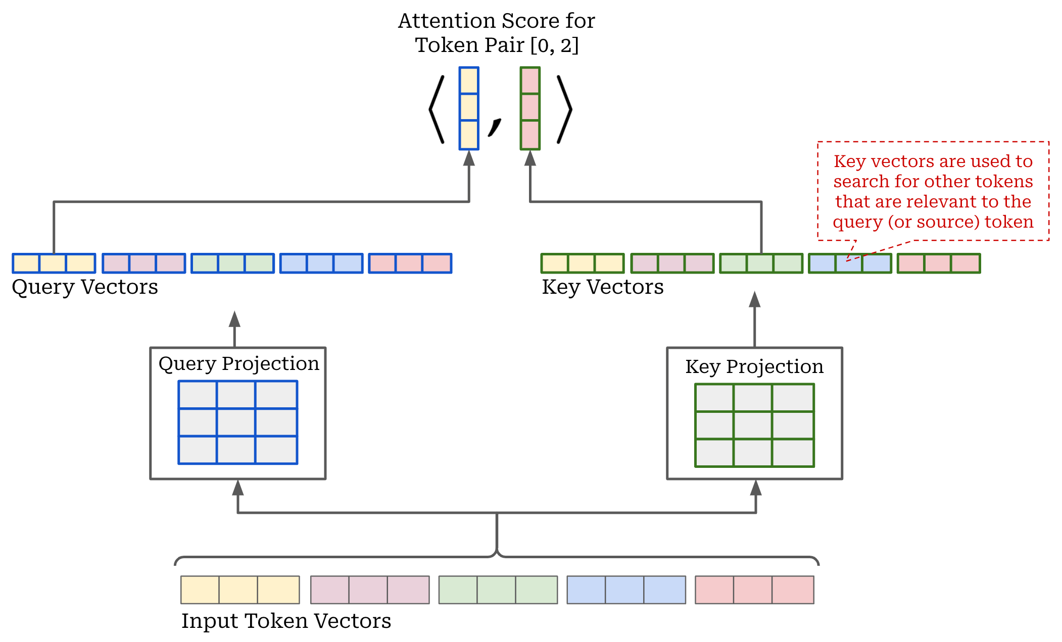
Scaled Dot Product Attention. Given our input token matrix of size [C, d] (i.e., we will assume that we are processing a single input sequence instead of a batch for simplicity), we begin by projecting our input using three separate linear projections, forming three separate sets of (transformed) token vectors. These projections are referred to as the key, query and value projections; see below.

Creating key, query and value vectors

This naming convention might seem random, but it comes from prior research in information retrieval. The intuitive reasoning for the name of each projection is as follows:

• A query is what you use to search for information. It represents the current token for which we want to find other relevant tokens in the sequence.

• The key represents each other token in the sequence and acts as an index to match the query with other relevant tokens in the sequence.

• The value is the actual information that is retrieved once a query matches a key. The value is used to compute each token’s output in self-attention.

Computing attention scores. After projecting the input, we compute an attention score a[i, j] for each pair of tokens [i, j] in our input sequence. Intuitively, this attention score, which lies in the [0, 1] range, captures how much a given token should “pay attention” to another token in the sequence—higher attention scores indicate that a pair of tokens are very relevant to each other. As hinted at above, attention scores are generated using the key and query vectors. We compute a[i, j] by taking the dot product of the query vector for token i with the key vector for token j; see below for a depiction of this process.

Computing an attention score for a token pair

We can efficiently compute all pairwise attention scores in a sequence by:

• Stacking the query and key vectors into two matrices.

• Multiplying the query matrix with the transposed key matrix.

This operation forms a matrix of size [C, C]—called the attention matrix—that contains all pairwise attention scores over the entire sequence. From here, we divide each value in the attention matrix by the square root of d—an approach that has been found to improve training stability [1]—and apply a softmax operation to each row of the attention matrix; see below. After softmax has been applied, each row of the attention matrix forms a valid probability distribution—each row contains positive values that sum to one. The i-th row of the attention matrix stores probabilities between the i-th token and each other token in our sequence.

Computing attention scores and output for self-attention

Computing output. Once we have the attention scores, deriving the output of self-attention is easy. The output for each token is simply a weighted combination of value vectors, where the weights are given by the attention scores. To compute this output, we simply multiply the attention matrix by the value matrix as shown above. Notably, self-attention preserves the size of its input—a transformed, d-dimensional output vector is produced for each token vector within the input.

Masked self-attention. So far, the formulation we have learned is for vanilla (or bidirectional self-attention). As mentioned previously, however, decoder-only transformers use masked self-attention, which modifies the underlying attention pattern by “masking out” tokens that come after each token in the sequence. Each token can only consider tokens that come before it—following tokens are masked.

Computing masked attention scores

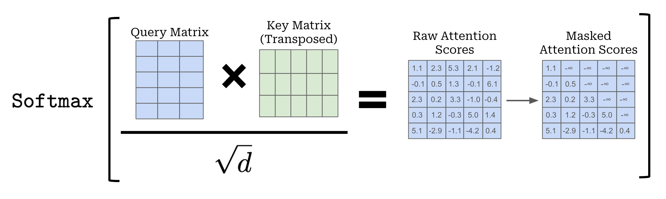
Let’s consider a token sequence [“LLM”, “#s”, “are”, “cool”, “.”] and compute masked attention scores for the token “are”. So far, we have learned that self-attention will compute an attention score between “are” and every other token in the sequence. With masked self-attention, however, we only compute attention scores for “LLM”, “#s”, and “are”. Masked self-attention prohibits us from looking forward in the sequence! Practically, this is achieved by simply setting all attention scores for these tokens to negative infinity, yielding a pairwise probability of zero for masked tokens after the application of softmax.

(from [1])

Attention heads. The attention operation we have described so far uses softmax to normalize attention scores that are computed across the sequence. Although this approach forms a valid probability distribution, it also limits the ability of self-attention to focus on multiple positions within the sequence—the probability distribution can easily be dominated by one (or a few) words. To solve this issue, we typically compute attention across multiple “heads” in parallel; see above.

Within each head, the masked attention operation is identical. However, we:

1. Use separate key, query, and value projections for each attention head.

2. Reduce the dimensionality of the key, query, and value vectors (i.e., this can be done by modifying the linear projection) to reduce computational costs.

More specifically, we will change the dimensionality of vectors in each attention head from d to d // H, where H is the number of attention heads, to keep the computational costs of multi-headed self-attention (relatively) fixed.

Combining the output of multiple attention heads

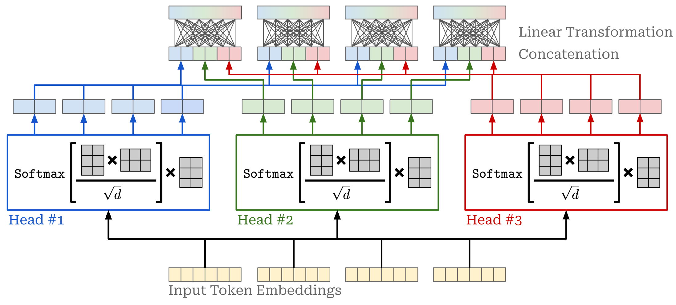
Now, we have several attention heads that compute self-attention in parallel. However, we still need to produce a single output representation from the multiple heads of our self-attention module. We have several options for combining the output of each attention head; e.g., concatenation, averaging, projecting, and more. However, the vanilla implementation of multi-headed self-attention does the following (depicted above):

• Concatenates the output of each head.

• Linearly projects the concatenated output.

Because each attention head outputs token vectors of dimension d // H, the concatenated output of all attention heads has dimension d . Thus, the multi-headed self-attention operation still preserves the original size of the input.

This file contains bidirectional Unicode text that may be interpreted or compiled differently than what appears below. To review, open the file in an editor that reveals hidden Unicode characters. Learn more about bidirectional Unicode characters

Show hidden characters

	"""
	Source: https://github.com/karpathy/nanoGPT/blob/master/model.py
	"""
	import math
	import torch
	from torch import nn
	import torch.nn.functional as F
	class CausalSelfAttention(nn.Module):
	def __init__(
	self,
	d,
	H,
	T,
	bias=False,
	dropout=0.2,
	):
	"""
	Arguments:
	d: size of embedding dimension
	H: number of attention heads
	T: maximum length of input sequences (in tokens)
	bias: whether or not to use bias in linear layers
	dropout: probability of dropout
	"""
	super().__init__()
	assert d % H == 0
	# key, query, value projections for all heads, but in a batch
	# output is 3X the dimension because it includes key, query and value
	self.c_attn = nn.Linear(d, 3*d, bias=bias)
	# projection of concatenated attention head outputs
	self.c_proj = nn.Linear(d, d, bias=bias)
	# dropout modules
	self.attn_dropout = nn.Dropout(dropout)
	self.resid_dropout = nn.Dropout(dropout)
	self.H = H
	self.d = d
	# causal mask to ensure that attention is only applied to
	# the left in the input sequence
	self.register_buffer("mask", torch.tril(torch.ones(T, T))
	.view(1, 1, T, T))
	def forward(self, x):
	B, T, _ = x.size() # batch size, sequence length, embedding dimensionality
	# compute query, key, and value vectors for all heads in batch
	# split the output into separate query, key, and value tensors
	q, k, v = self.c_attn(x).split(self.d, dim=2) # [B, T, d]
	# reshape tensor into sequences of smaller token vectors for each head
	k = k.view(B, T, self.H, self.d // self.H).transpose(1, 2) # [B, H, T, d // H]
	q = q.view(B, T, self.H, self.d // self.H).transpose(1, 2)
	v = v.view(B, T, self.H, self.d // self.H).transpose(1, 2)
	# compute the attention matrix, perform masking, and apply dropout
	att = (q @ k.transpose(-2, -1)) * (1.0 / math.sqrt(k.size(-1))) # [B, H, T, T]
	att = att.masked_fill(self.mask[:,:,:T,:T] == 0, float('-inf'))
	att = F.softmax(att, dim=-1)
	att = self.attn_dropout(att)
	# compute output vectors for each token
	y = att @ v # [B, H, T, d // H]
	# concatenate outputs from each attention head and linearly project
	y = y.transpose(1, 2).contiguous().view(B, T, self.d)
	y = self.resid_dropout(self.c_proj(y))
	return y

view raw causal_self_attention.py hosted with ❤ by GitHub

Full implementation. A full implementation of masked multi-headed self-attention is provided above. Here, we go beyond a single input sequence of size [C, d] and process a batch of inputs of size [B, C, d]. The above code implements each of the components that we have described so far:

• Lines 52-59: compute key, query and value projections (using a single linear projection) for each attention head and split / reshape them as necessary.

• Lines 62-65: compute attention scores, mask the attention scores, then apply a softmax transformation to the result⁴.

• Line 68: compute output vectors by taking the product of the attention matrix and the value matrix.

• Lines 71-72: concatenate the outputs from each attention head and apply a linear projection to form the final output.

Although we use some fancy matrix manipulations and operations in PyTorch, this implementation exactly matches our description of masked self-attention!

Feed-Forward Transformation

Pointwise feed-forward transformation

In addition to masked self-attention, each block of the transformer contains a pointwise⁵ feed-forward transformation; see above. This transformation passes each token vector within the sequence through the same feed-forward neural network. Usually, this is a two-layer network with a non-linear activation (e.g., ReLU, GeLU or SwiGLU [3]) in the hidden layer. In most cases, the dimension of the hidden layer is larger than the original dimension of our token embeddings (e.g., by 4×). Implementing a feed-forward neural network in PyTorch is easy to accomplish with the Linear module; see below for an example.

This file contains bidirectional Unicode text that may be interpreted or compiled differently than what appears below. To review, open the file in an editor that reveals hidden Unicode characters. Learn more about bidirectional Unicode characters

Show hidden characters

	"""
	Source: https://github.com/karpathy/nanoGPT/blob/master/model.py
	"""
	from torch import nn
	class MLP(nn.Module):
	def __init__(
	self,
	d,
	bias=False,
	dropout=0.2
	):
	"""
	Arguments:
	d: size of embedding dimension
	bias: whether or not to use bias in linear layers
	dropout: probability of dropout
	"""
	super().__init__()
	self.c_fc = nn.Linear(d, 4 * d, bias=bias)
	self.gelu = nn.GELU()
	self.c_proj = nn.Linear(4 * d, d, bias=bias)
	self.dropout = nn.Dropout(dropout)
	def forward(self, x):
	x = self.c_fc(x)
	x = self.gelu(x)
	x = self.c_proj(x)
	x = self.dropout(x)
	return x

view raw transformer_ffnn.py hosted with ❤ by GitHub

Decoder-Only Transformer Block

Decoder-only Transformer Block

To construct a decoder-only transformer block, we use both components—masked self-attention and a feed-forward transformation—that we have seen so far, as well as place normalization operations and residual connections between components. A depiction of the full decoder-only transformer block⁶ is shown above.

A residual connection [4] simply adds the input for a neural network layer to the output for that layer before passing this representation to the next layer—as opposed to solely passing the layer’s output to the next layer without adding the input.

Residual connection in a generic neural network layer

Residual connections are widely used within deep learning and can be applied to any kind of neural network layer⁷. Adding residual connections helps to avoid issues with vanishing / exploding gradients and generally improves the stability of training by providing a “short cut” that allows gradients to flow freely through the network during backpropagation; see here for more details.

Layer normalization with an affine transformation

Normalizing the input (or output) of a neural network layer can also aid training stability. Although many types of normalization exist, the most commonly used normalization variant for transformers / LLMs is layer normalization; see above. Here, the normalization operation has two components:

1. Performing normalization.

2. Applying a (learnable) affine transformation.

In other words, we multiply the normalized values by weight and add a bias instead of directly using the normalized output. Both the weight and bias are learnable parameters that can be trained along with other network parameters. Layer normalization is implemented in PyTorch and easy to use; see here.

This file contains bidirectional Unicode text that may be interpreted or compiled differently than what appears below. To review, open the file in an editor that reveals hidden Unicode characters. Learn more about bidirectional Unicode characters

Show hidden characters

	"""
	Source: https://github.com/karpathy/nanoGPT/blob/master/model.py
	"""
	from torch import nn
	class Block(nn.Module):
	def __init__(
	self,
	d,
	H,
	T,
	bias=False,
	dropout=0.2,
	):
	"""
	Arguments:
	d: size of embedding dimension
	H: number of attention heads
	T: maximum length of input sequences (in tokens)
	bias: whether or not to use bias in linear layers
	dropout: probability of dropout
	"""
	super().__init__()
	self.ln_1 = nn.LayerNorm(d)
	self.attn = CausalSelfAttention(d, H, T, bias, dropout)
	self.ln_2 = nn.LayerNorm(d)
	self.ffnn = MLP(d, bias, dropout)
	def forward(self, x):
	x = x + self.attn(self.ln_1(x))
	x = x + self.ffnn(self.ln_2(x))
	return x

view raw decoder_only_block.py hosted with ❤ by GitHub

Block implementation. A decoder-only transformer block implementation is provided above. Here, we use our prior attention and feed-forward transformation implementations. By using the modules we have already defined, the decoder-only transformer block implementation actually becomes quite simple!

Decoder-only Transformer Architecture

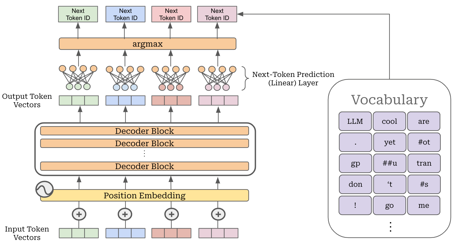
Once we grasp the input and block structure of the decoder-only transformer, the rest of the architecture is pretty simple—we just repeat the same block L times! For each block, the size of the model’s input [B, C, d] is maintained, so the output of our L-th decoder-only transformer block is also a tensor of this size; see below.

Predicting next tokens with an LLM

A full implementation of a (GPT-style) decoder-only transformer architecture is provided below. Here, the architecture contains several components, including two embedding layers (i.e., for tokens and positions), all L transformer blocks, and a final classification module—including layer normalization and a linear layer—for performing next token prediction given an output token embedding as input. The model operates by just passing its input—a set of input token IDs with size [B, C]—through each of these components to produce a set of output token IDs.

This file contains bidirectional Unicode text that may be interpreted or compiled differently than what appears below. To review, open the file in an editor that reveals hidden Unicode characters. Learn more about bidirectional Unicode characters

Show hidden characters

	"""
	Source: https://github.com/karpathy/nanoGPT/blob/master/model.py
	"""
	import torch
	from torch import nn
	import torch.nn.functional as F
	class GPT(nn.Module):
	def __init__(self,
	d,
	H,
	C,
	V,
	layers,
	bias=False,
	dropout=0.2,
	):
	"""
	Arguments:
	d: size of embedding dimension
	H: number of attention heads
	C: maximum length of input sequences (in tokens)
	V: size of the token vocabulary
	layers: number of decoder-only blocks
	bias: whether or not to use bias in linear layers
	dropout: probability of dropout
	"""
	super().__init__()
	self.transformer = nn.ModuleDict(dict(
	wte=nn.Embedding(V, d), # token embeddings
	wpe=nn.Embedding(C, d), # position embeddings
	drop=nn.Dropout(dropout),
	blocks=nn.ModuleList([Block(d, H, C, bias, dropout) for _ in range(layers)]),
	ln_f=nn.LayerNorm(d),
	head=nn.Linear(d, V, bias=bias),
	))
	def forward(self, idx, targets=None):
	# idx is a [B, C] matrix of token indices
	# targets is a [B, C] matrix of target (next) token indices
	device = idx.device
	_, C = idx.size() # [B, C]
	pos = torch.arange(0, C, dtype=torch.long, device=device)
	# generate token and position embeddings
	tok_emb = self.transformer.wte(idx) # [B, C, d]
	pos_emb = self.transformer.wpe(pos) # [C, d]
	x = self.transformer.drop(tok_emb + pos_emb)
	# pass through all decoder-only blocks
	for block in self.transformer.blocks:
	x = block(x)
	x = self.transformer.ln_f(x) # final layer norm
	if targets is not None:
	# compute the loss if we are given targets
	logits = self.transformer.head(x)
	loss = F.cross_entropy(
	logits.view(-1, logits.size(-1)),
	targets.view(-1),
	ignore_index=-1,
	)
	else:
	# only look at last token if performing inference
	logits = self.transformer.head(x[:, [-1], :])
	loss = None
	return logits, loss

view raw gpt.py hosted with ❤ by GitHub

Generating output (decoding). LLMs are trained specifically to perform next-token prediction. In other words, these models are specialists in predicting the next token given a list of tokens as input. As we have learned, the model’s output is just a list of output token vectors corresponding to each input token. So, we can predict the next token for any of these inputs tokens by:

1. Taking the output embedding for a particular token.

2. Passing this embedding through a linear layer, where the output size is the dimension of the model’s vocabulary.

3. Taking an argmax of the model’s output to get the maximum token ID.

To generate a sequence of text, we just continue to repeat this process. We ingest a textual prompt as input, pass everything through the decoder-only transformer, take the last token vector in our output sequence, predict the next token, add this next token to our input sequence and repeat. This autoregressive decoding process is used by all LLMs to generate their output; see below.

Autoregressive output generation with next token prediction

Why the decoder? Now that we understand this architecture, we might wonder: Why do LLMs only use the decoder component of the transformer? The key distinction between the encoder and decoder for a transformer is the type of attention that is used. The encoder uses bidirectional self-attention, meaning all tokens in the sequence—including those before and after a given token—are considered by the self-attention mechanism. In contrast, the decoder uses masked self-attention, which prevents tokens from attending to those that follow them in the sequence.

Causal mask for next token prediction

Due to the use of masked self-attention, decoders work well for next token prediction. If each token can look forward in the sequence when crafting its representation, then the model could simply learn to predict next tokens by cheating (i.e., directly copying the next token in the sequence); see above. Masked self-attention forces the model to learn generalizable patterns for predicting next tokens from those that come before them, making the decoder perfect for LLMs.

Creating a Mixture-of-Experts (MoE) Model

“In deep learning, models typically reuse the same parameters for all inputs. Mixture of Experts (MoE) models defy this and instead select different parameters for each incoming example. The result is a sparsely-activated model—with an outrageous number of parameters—but a constant computational cost.” - from [6]

Now that we have an in-depth understanding of decoder-only transformers, we need to create a Mixture-of-Experts (MoE) model. MoE-based LLMs maintain the same decoder-only transformer architecture, but they modify this architecture in a few subtle ways. See the posts below for an in-depth coverage of these ideas.

Mixture-of-Experts (MoE): The Birth and Rise of Conditional Computation

Mixture-of-Experts (MoE) LLMs

Converting the model architecture to an MoE is not that difficult, but there are a lot of small details that must be implemented correctly for the model to work well. Additionally, training these models properly requires some extra attention and understanding—MoE models are more difficult to train than a standard LLM.

Expert Layers

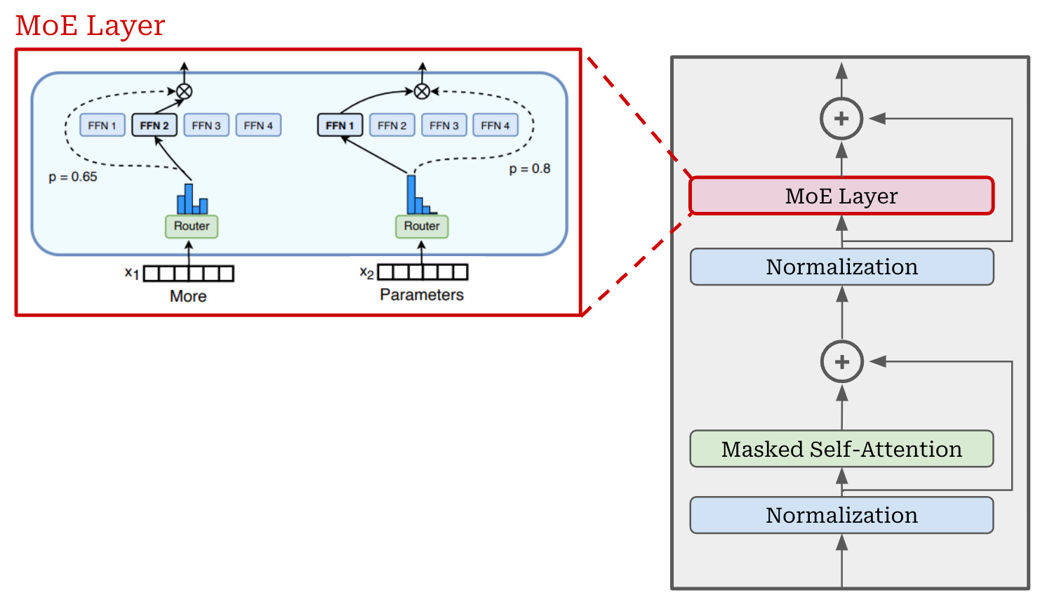
Compared to the standard decoder-only transformer, the main modification made by an MoE model is within the feed-forward component of the transformer block. Usually, this block has one feed-forward network that is applied in a pointwise fashion across all token vectors. Instead of having a single feed-forward network, an MoE creates several feed-forward networks, each with their own independent weights. We refer to each of these networks as an “expert”, and a feed-forward layer with several experts is called an “expert layer”. If we have N experts in a layer, we can refer to the i-th expert using the notation E_i; see below.

PyTorch Implementation. Implementing an expert layer in PyTorch is not that complicated. As shown below, we just use our same implementation from before, but create several feed-forward networks instead of one. The main complexity to this implementation is that we do not use standard Linear layers in PyTorch. Instead, we wrap the weights of all experts into several Parameter objects so that we can compute the output of all experts in batch by using the batch matrix multiplication operator. This implementation avoids having to loop over each expert to compute its output, which drastically improves efficiency.

This file contains bidirectional Unicode text that may be interpreted or compiled differently than what appears below. To review, open the file in an editor that reveals hidden Unicode characters. Learn more about bidirectional Unicode characters

Show hidden characters

	"""
	Based upon ColossalAI OpenMoE: https://github.com/hpcaitech/ColossalAI/blob/main/colossalai/moe/experts.py
	"""
	import torch
	from torch import nn
	class MLPExperts(nn.Module):
	def __init__(
	self,
	d,
	n_exp=8,
	bias=False,
	dropout=0.2,
	):
	"""
	Arguments:
	d: size of embedding dimension
	n_exp: the number of experts to create in the expert layer
	bias: whether or not to use bias in linear layers
	dropout: probability of dropout
	"""
	super().__init__()
	self.bias = bias
	self.c_fc = nn.Parameter(torch.empty(n_exp, d, 4 * d))
	self.c_proj = nn.Parameter(torch.empty(n_exp, 4 * d, d))
	self.fc_bias = nn.Parameter(torch.empty(n_exp, 1, 4 * d)) if self.bias else None
	self.proj_bias = nn.Parameter(torch.empty(n_exp, 1, d)) if self.bias else None
	self.gelu = nn.GELU()
	self.dropout = nn.Dropout(dropout)
	def forward(self, x):
	x = torch.bmm(x, self.c_fc)
	if self.bias:
	x += self.fc_bias
	x = self.gelu(x)
	x = torch.bmm(x, self.c_proj)
	if self.bias:
	x += self.proj_bias
	x = self.dropout(x)
	return x

view raw expert_layer.py hosted with ❤ by GitHub

Creating an MoE. To create an MoE-based decoder-only transformer, we simply convert the transformer’s feed-forward layers to MoE—or expert—layers. Each expert within the MoE layer has an architecture that is identical to the original, feed-forward network from that layer. We just have several independent copies of the original feed-forward network within an expert layer; see below.

Adding experts to a decoder-only transformer (from [1])

However, we need not use experts for every feed-forward layer in the transformer. Most MoE-based LLMs use a stride of P, meaning that every P-th layer is converted into an expert layer and other layer are left untouched.

“The ST-MoE models have 32 experts with an expert layer frequency of 1/4 (every fourth FFN layer is replaced by an MoE layer).” - from [24]

A high-level implementation of this idea is provided in the pseudocode shown below. These “interleaved” MoE layers control the total number of experts within the MoE, which is a useful mechanism for balancing performance and efficiency.

transformer_blocks = []
for i in range(num_blocks):
    use_moe = (i % P) == 0

    # when use_moe = False, this is regular transformer block
    # when use_moe = True, this is an expert layer
    transformer_blocks.append(Block(use_moe=use_moe))

Routing Tokens to Experts

The primary benefit of MoE-based architectures is their efficiency, but using experts alone does not improve efficiency! In fact, adding more experts to each layer of the model significantly increases the total number parameters—and the amount of necessary compute—for the model. To improve efficiency, we need to sparsely select and use only a subset of experts within each layer. By sparsely utilizing experts, we can get the benefits of a much larger model without a significant increase in the computational costs of training and inference.

“Using an MoE architecture makes it possible to attain better tradeoffs between model quality and inference efficiency than dense models typically achieve.” - source

Selecting experts. Let’s consider a single token—represented by a d-dimensional token vector. Our goal is to select a subset of experts (of size k) to process this token. In the MoE literature, we usually say that the token will be “routed” to these experts. We need an algorithm to compute and optimize this routing operation.

Routing mechanism for a single token

The simplest possible routing algorithm would apply a linear transformation to the token vector, forming a vector of size N (i.e., the number of experts). Then, we can apply a softmax function to form a probability distribution over the set of experts for our token; see above. We can use this distribution to choose experts to which our token should be routed by selecting top-K experts in the distribution. The top-K values—the “expert probabilities”—are also important.

Simple router implementation. As described above, this routing mechanism is actually quite simple—it’s just a linear layer! An implementation of this softmax router is shown below, where the output of our router is:

1. A set of top-K expert indices for each token in the input.

2. The top-K expert probabilities (i.e., the probability values for each of the top-K indices) associated with selected experts.

Despite its simplicity, this routing mechanism is effective and serves its purpose well. Most modern MoEs adopt a similar linear routing scheme with softmax.

This file contains bidirectional Unicode text that may be interpreted or compiled differently than what appears below. To review, open the file in an editor that reveals hidden Unicode characters. Learn more about bidirectional Unicode characters

Show hidden characters

	import torch
	from torch import nn
	from torch.nn import functional as F
	class BasicSoftmaxRouter(nn.Module):
	def __init__(
	self,
	d,
	n_exp = 8,
	top_k = 2,
	use_noisy_top_k = True,
	):
	"""
	Arguments:
	d: size of embedding dimension
	n_exp: the number of experts to create in the expert layer
	top_k: the number of active experts for each token
	use_noisy_top_k: whether to add noise when computing expert output
	"""
	super().__init__()
	# router settings
	self.top_k = top_k
	assert self.top_k >= 1 and self.top_k <= n_exp
	self.use_noisy_top_k = use_noisy_top_k
	# linear projection for (noisy) softmax routing
	# no bias used, see page 4 eq (4) in https://arxiv.org/abs/1701.06538
	self.w_g = nn.Linear(d, n_exp, bias=False)
	self.w_noise = nn.Linear(d, n_exp, bias=False) if self.use_noisy_top_k else None
	def forward(self, x):
	# eq (4) in https://arxiv.org/abs/1701.06538
	logits = self.w_g(x) # [B, C, d] -> [B, C, n_exp]
	if self.use_noisy_top_k:
	# (optionally) add noise into the router
	noise = F.softplus(self.w_noise(x))
	noise *= torch.randn_like(noise)
	logits += noise
	top_k_logits, top_k_indices = logits.topk(self.top_k, dim=-1) # [B, C, k]
	return top_k_logits, top_k_indices

view raw basic_softmax_router.py hosted with ❤ by GitHub

Optionally, we can add noise into the routing mechanism, an approach proposed in [8]—one of the earliest works on applying MoEs to neural networks. By adding this small amount of (learnable) noise into the output of the routing mechanism (see below for details), we can help to regularize the MoE’s training process.

Adding noise to top-k softmax routing (from [7])

Active parameters. Because we only select a subset of experts to process each token within an MoE layer, there is a concept of “active” parameters in the MoE literature. Put simply, only a small portion of the MoE model’s total parameters—given by the experts selected at each MoE layer—are active when processing a given token. The total computation performed by the MoE is proportional to the number of active parameters rather than the total number of parameters.

Expert Capacity

“To improve hardware utilization, most implementations of sparse models have static batch sizes for each expert. The expert capacity refers to the number of tokens that can be routed to each expert. If this capacity is exceeded then the overflowed tokens… are passed to the next layer through a residual connection.” - from [5]

The computation performed in an expert layer is dynamic. We choose the tokens to be computed by each expert based on the output of the router, which changes depending upon the sequences of tokens provided as input to the MoE. The dynamic nature of the input for each expert can make the implementation of an expert layer somewhat complicated: How can we deal with the fact that each expert’s input will have a different and unpredictable size?

Computing the expert capacity

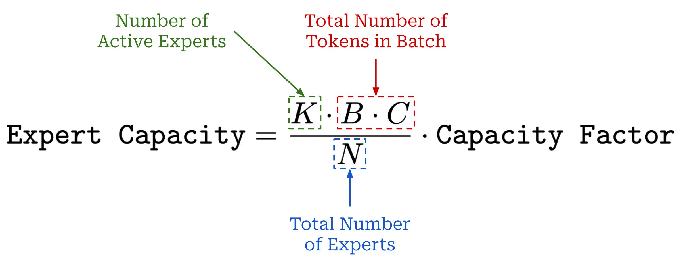
Expert capacity. Most practical implementations of MoEs avoid this problem by using fixed batch sizes for each expert—this is a useful trick for improving hardware utilization. Each expert uses the same static batch size, referred to as “expert capacity”. The expert capacity—defined in the above equation—dictates the maximum number of tokens in each batch that can be sent to any single expert.

Expert capacity is controlled via the capacity factor setting. A capacity factor of one means that tokens are routed uniformly, while setting the capacity factor greater than one provides extra buffer to handle imbalanced token routing between experts—this comes at the cost of higher memory usage and lower efficiency.

(from [6])

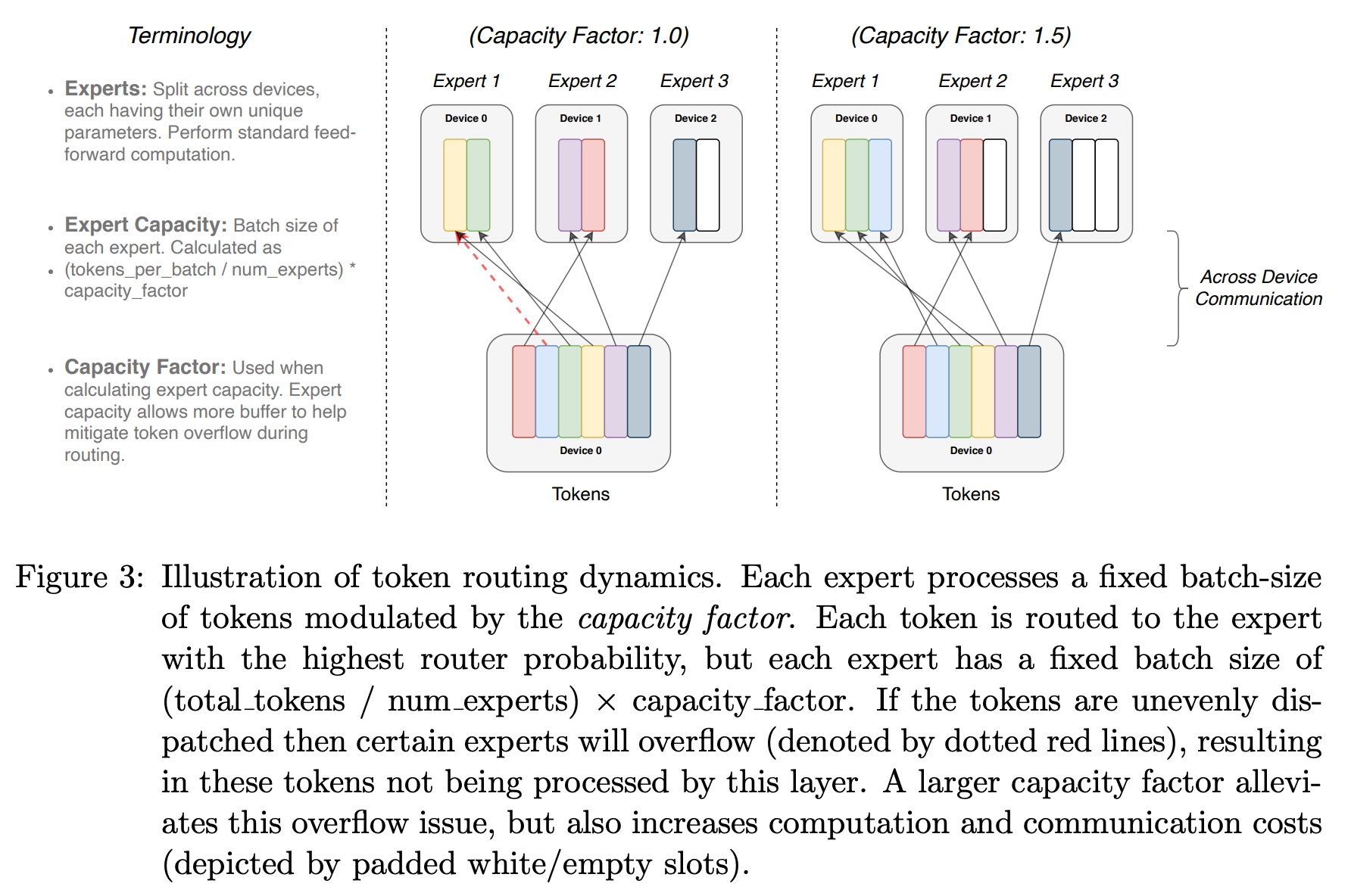
If the number of tokens routed to an expert exceeds the expert capacity, then we “drop” these extra tokens by performing no computation and letting their representation flow directly to the next layer via the transformer’s residual connection; see above. MoEs perform well with relatively low capacity factors⁸, but we should make sure to avoid too many tokens being dropped. The capacity factor can also be different during training and evaluation; e.g., ST-MoE [5] uses a capacity factor of 1.25 and 2.0 during training and evaluation, respectively.

PyTorch implementation. Now that we understand expert capacity and the details of routing within an expert layer, we need to implement a fully-functional router. This router will share the same logic as our prior implementation (i.e., a linear layer with softmax), but it will go beyond this implementation by creating the fixed-size input tensors for each of the experts; see below. Given that this is a fully-functional implementation, the router below is more complex than before. However, we can distill this implementation into the following components:

• Lines 41-47: Compute the output of the (noisy) linear router.

• Lines 49-52: Compute the top-K experts and their associated probabilities.

• Lines 55-58: Compute the expert capacity.

• Lines 60-88: Use fancy PyTorch indexing and tensor manipulation to handle constructing the batch of expert inputs⁹.

• Lines 90-93: Construct the final batch of expert inputs.

This file contains bidirectional Unicode text that may be interpreted or compiled differently than what appears below. To review, open the file in an editor that reveals hidden Unicode characters. Learn more about bidirectional Unicode characters

Show hidden characters

	import math
	import torch
	from torch import nn
	from torch.nn import functional as F
	class Router(nn.Module):
	def __init__(
	self,
	d,
	n_exp = 8,
	top_k = 2,
	use_noisy_top_k = True,
	capacity_factor = 1.25,
	):
	"""
	Arguments:
	d: size of embedding dimension
	n_exp: the number of experts to create in the expert layer
	top_k: the number of active experts for each token
	use_noisy_top_k: whether to add noise when computing expert output
	capacity_factor: used to compute expert capacity
	"""
	super().__init__()
	self.d = d
	self.n_exp = n_exp
	self.top_k = top_k
	assert self.top_k >= 1 and self.top_k <= n_exp
	self.use_noisy_top_k = use_noisy_top_k
	self.capacity_factor = capacity_factor
	self.w_g = nn.Linear(d, n_exp, bias=False)
	self.w_noise = nn.Linear(d, n_exp, bias=False) if self.use_noisy_top_k else None
	def forward(self, x):
	# get the total number of tokens in the batch
	B, C, _ = x.size()
	num_tokens = B * C
	# eq (4) in https://arxiv.org/abs/1701.06538
	logits = self.w_g(x) # [B, C, d] -> [B, C, n_exp]
	if self.use_noisy_top_k:
	# (optionally) add noise into the router
	noise = F.softplus(self.w_noise(x))
	noise *= torch.randn_like(noise)
	logits += noise
	# top-K expert selection, compute probabilities over active experts
	top_k_logits, top_k_indices = logits.topk(self.top_k, dim=-1) # [B, C, K]
	router_probs = torch.full_like(logits, float('-inf')) # [B, C, n_exp]
	router_probs.scatter_(-1, top_k_indices, top_k_logits)
	router_probs = F.softmax(router_probs, dim=-1)
	# compute the expert capacity
	exp_capacity = math.floor(self.top_k * self.capacity_factor * num_tokens / self.n_exp)
	exp_capacity += exp_capacity % 2 # make sure expert capacity is an even integer
	exp_capacity = int(exp_capacity)
	# make a multi-hot mask of chosen experts
	# values are 0 if expert not chosen, 1 if expert chosen
	exp_mask = F.one_hot(top_k_indices, num_classes=self.n_exp) # [B, C, K, n_exp]
	exp_mask = exp_mask.view(num_tokens, self.top_k, self.n_exp) # [B * C, K, n_exp]
	exp_mask = exp_mask.permute(1, 0, 2) # [K, B * C, n_exp]
	# compute index for each token in expert batch
	# NOTE: cumsum counts top-1 first, top-2 second, etc.
	# to prioritize top experts when dropping tokens
	exp_rank = exp_mask.reshape(self.top_k * num_tokens, self.n_exp) # [K * B * C, n_exp]
	exp_rank = torch.cumsum(exp_rank, dim=0) - 1 # cumsum of expert selections [K * B * C, n_exp]
	exp_rank = exp_rank.reshape(self.top_k, num_tokens, self.n_exp) # [K, B * C, n_exp]
	# mask entries beyond expert capacity and compute used capacity
	exp_mask *= torch.lt(exp_rank, exp_capacity) # [K, B * C, n_exp]
	# matrix storing token position in batch of corresponding expert
	exp_rank = torch.sum(exp_mask * exp_rank, dim=-1) # [K, B * C]
	# mask probabilities to only include selected experts
	router_probs = router_probs.view(num_tokens, self.n_exp)[None, :] # [1, B * C, n_exp]
	exp_weights = exp_mask * router_probs # [K, B * C, n_exp]
	# position of each token within the capacity of the selected expert
	exp_rank_sc = F.one_hot(exp_rank, num_classes=exp_capacity) # [K, B * C, exp_capacity]
	# weight of selected expert for each token at position the capacity of that expert
	exp_weights = torch.sum(exp_weights.unsqueeze(3) * exp_rank_sc.unsqueeze(2), dim=0) # [B * C, n_exp, exp_capacity]
	exp_mask = exp_weights.bool() # binary mask of selected experts for each token
	# reshape tokens into batches for each expert, return both weights and batches
	# [n_exp, exp_capacity, B * C] * [B * C, d] -> [n_exp, exp_capacity, n_embd]
	x = x.view(num_tokens, self.d)
	expert_batches = exp_mask.permute(1, 2, 0).type_as(x) @ x
	return exp_weights, exp_mask, expert_batches

view raw full_softmax_router.py hosted with ❤ by GitHub

Load Balancing and Auxiliary Losses

“The gating network tends to converge to a state where it always produces large weights for the same few experts. This imbalance is self-reinforcing, as the favored experts are trained more rapidly and thus are selected even more by the gating network.” - from [7]

So far, the routing system we have devised does not explicitly encourage a balanced selection of experts in each layer. As a result, the model will converge to a state of repeatedly selecting the same few experts for every token instead of fully utilizing its experts. This phenomenon, which is explained in the quote above, is commonly referred to as “routing collapse”.

(from [6])

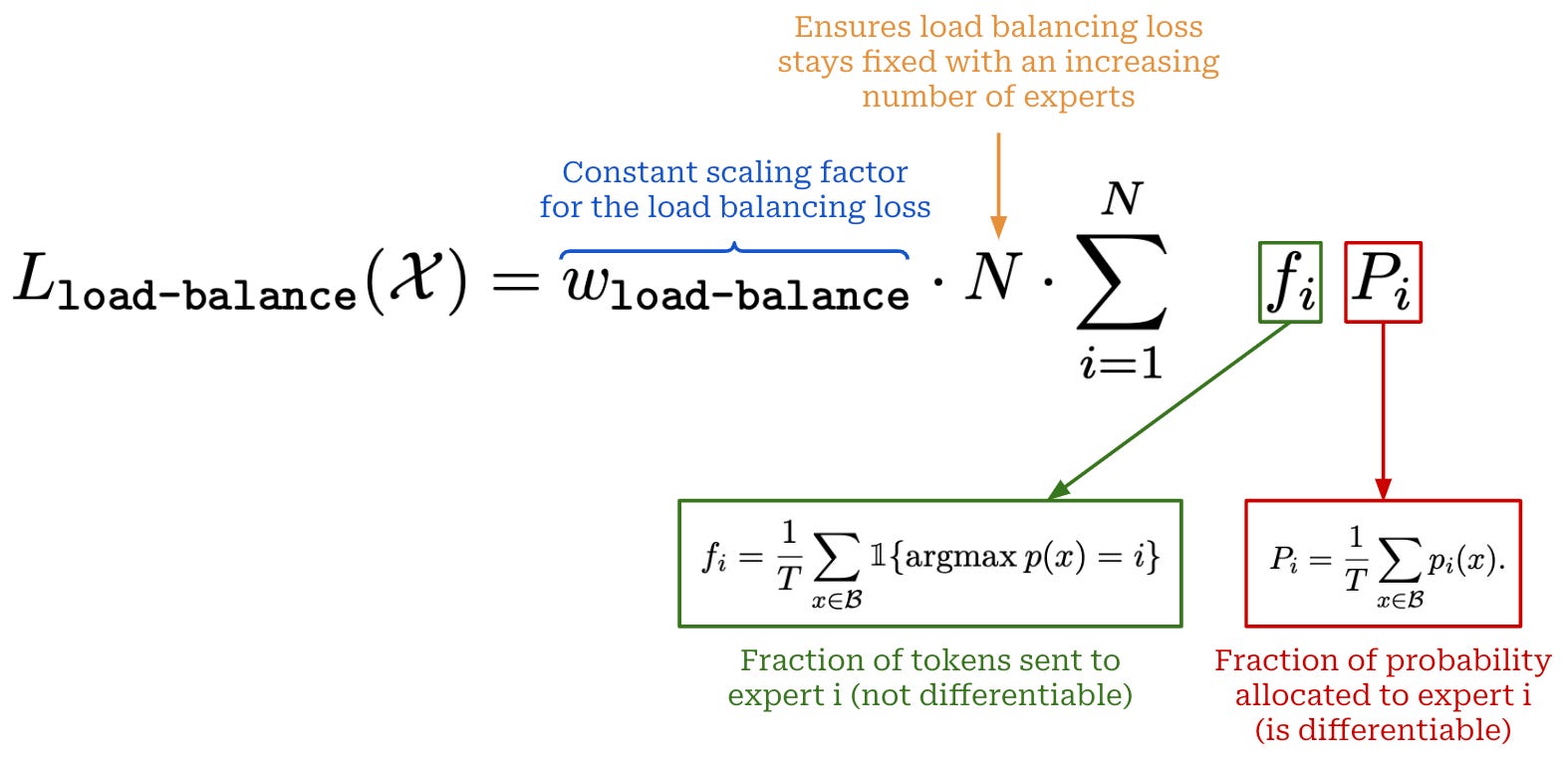
Load balancing loss. To encourage a balanced selection of experts during training, we can simply add an additional component to the training loss that rewards the model for uniformly leveraging its experts. More specifically, we create the auxiliary loss term shown above, which measures expert importance (i.e., the probability assigned to each expert) and load balancing (i.e., the number of tokens sent to each expert). Such an approach is proposed in [2], where authors create a loss that considers two quantities:

1. The fraction of router probability allocated to each expert¹⁰.

2. The fraction of tokens dispatched to each expert.

If we store both of these quantities in their own N-dimensional vectors, we can create a single loss term by taking the dot product of these two vectors. This loss is minimized when experts receive uniform probability and load balancing.

An implementation of this load balancing loss in PyTorch is provided below. This implementation has the following key components:

• Lines 9-17: define all constants and input tensors used for computing the load balancing loss.

• Lines 19-24: compute the ratio or fraction of tokens sent to each expert.

• Lines 26-27: compute the fraction of probability allocated to each expert.

• Lines 29-31: take a (scaled) dot product between the ratio of tokens and probability for each expert¹¹.

This file contains bidirectional Unicode text that may be interpreted or compiled differently than what appears below. To review, open the file in an editor that reveals hidden Unicode characters. Learn more about bidirectional Unicode characters

Show hidden characters

	"""
	Computes Switch Transformer auxiliary loss (https://arxiv.org/abs/2101.03961)
	See equations (4)-(6) on page 7
	"""
	import torch
	import torch.nn.functional as F
	# constants
	B = 16 # batch size
	C = 256 # sequence length
	n_exp = 8 # number of experts
	K = 2 # number of active expert
	# define tensors needed to compute load balancing loss
	indices = torch.randint(1, n_exp + 1, (B, C, K)) # top-K indices ([B, C, K])
	expert_probs = F.softmax(torch.rand(B, C, n_exp), dim=2) # expert probabilities ([B, C, n_exp])
	# equation (5): compute ratio of tokens allocated to each expert
	# total number of tokens is defined as total tokens in batch * K
	with torch.no_grad():
	one_hot_indices = F.one_hot(indices, num_classes=n_exp) # [B, C, K, n_exp]
	one_hot_indices = torch.sum(one_hot_indices.float(), dim=2) # [B, C, n_exp] (sum over K dimension)
	tokens_per_expert = torch.mean(one_hot_indices.float(), dim=(0, 1))
	# equation (6): compute ratio of router probability allocated to each expert
	prob_per_expert = torch.mean(expert_probs.float(), dim=(0, 1))
	# equation (4): take a scaled dot product between prob / token allocation vectors
	# multiply the result by the number of experts
	load_balance_loss = n_exp * torch.sum(prob_per_expert * tokens_per_expert)

view raw load_balancing_loss.py hosted with ❤ by GitHub

Router z-loss. To complement the load balancing loss, authors in [3] propose an extra auxiliary loss term, called the router z-loss. The router z-loss constrains the size of the logits—not probabilities, this is before softmax is applied—predicted by the routing mechanism; see below for the formulation.

We do not want these logits to be too large due to the fact that the router contains an (exponential) softmax function. However, these logits can become very large during training, which can lead to round-off errors that destabilize the training process—even when using full (float32) precision. The router z-loss encourages the MoE to keep these logits small and, in turn, avoid these round-off errors.

“The router computes the probability distribution over the experts in float32 precision. However, at the largest scales, we find this is insufficient to yield reliable training.” - from [3]

An implementation of the router z-loss is provided below, which contains three key steps:

1. Lines 8-14: Create the input tensor needed to compute the router z-loss (i.e., logits from the routing mechanism).

2. Line 21: Take a squared logsumexp of router logits. This is a numerically stable shorthand for applying the exponential, sum, and log operations in sequence.

3. Line 24: Sum the result of the above operation over all tokens and divide by the total number of tokens (i.e., take an average).

This file contains bidirectional Unicode text that may be interpreted or compiled differently than what appears below. To review, open the file in an editor that reveals hidden Unicode characters. Learn more about bidirectional Unicode characters

Show hidden characters

	"""
	Computes ST-MoE router z loss (https://arxiv.org/abs/2202.08906)
	See equation (5) on page 7
	"""
	import torch
	# constants
	B = 16 # batch size
	C = 256 # sequence length
	n_exp = 8 # number of experts
	# create input tensor for router z-loss
	router_logits = torch.rand(B, C, n_exp) # [B, C, n_exp]
	# exponentiate logits, sum logits of each expert, take log, and square
	# code below is equivalent to the following:
	# z_loss = torch.exp(router_logits)
	# z_loss = torch.sum(z_loss, dim=-1)
	# z_loss = torch.log(z_loss) ** 2.0
	router_z_loss = torch.logsumexp(router_logits, dim=-1) ** 2.0 # [B, C]
	# sum over all tokens and divide by total number of tokens
	router_z_loss = torch.mean(router_z_loss)

view raw router_z_loss.py hosted with ❤ by GitHub

Combining auxiliary losses. Given that several auxiliary losses exist, we might wonder which of them we should use in practice. The answer is: all of them! We can just add each of these losses to our standard language modeling loss during training. Each auxiliary loss will have a scaling factor by which it is multiplied, then we sum all of the (scaled) losses together; see below. Default scaling factors for load balancing and router z-losses are 0.001 and 0.01, respectively.

Current research. As we will see, the auxiliary losses that we have learned about in this section work quite well. However, recent research [8] has shown that—depending upon how the scaling factors are set—such auxiliary losses might sacrifice model performance for training stability in some cases. As such, the optimal process and strategies for training MoEs is still a (very) active research area.

Auxiliary-loss-free load balancing from DeepSeek-v3 [8]

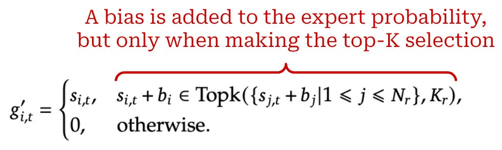
For example, the recently-proposed DeepSeek-v3 [8] model—the base model used to create the DeepSeek-R1 reasoning model—uses an auxiliary-loss-free load balancing strategy, which simply adds a dynamic bias to the router output when selecting top-K experts; see above. This bias is increased for experts that are not selected enough and decreased for experts that are selected too much, thus increasing the chance that under-utilized experts will be selected. This dynamic bias is found to improve load balancing without sacrificing model performance. However, load balancing losses are still used in [8] (just with a smaller scaling factor).

“We keep monitoring the expert load on the whole batch of each training step. At the end of each step, we will decrease the bias term by 𝛾 if its corresponding expert is overloaded, and increase it by 𝛾 if its corresponding expert is underloaded, where 𝛾 is a hyper-parameter called bias update speed.” - from [8]

Decoder-Only MoE Implementation

MoE-based Decoder-only Transformer Architecture

We now understand all of the major components of an expert layer. So, let’s put these concepts together to create a full MoE-based decoder-only architecture. The MoE blocks within this model (shown above) will contain:

• A regular (masked) self-attention layer

• An expert layer—instead of the normal feed-forward layer—for every P-th layer of the model.

This block structure is similar to that of a standard, decoder-only transformer, but we replace the feed-forward layer with an expert layer—forming an MoE block—in a portion of the model’s layers. First, let’s cover a few remaining details regarding how the final output of an expert layer is computed. Then, we will present a full implementation of the MoE-based decoder-only transformer.

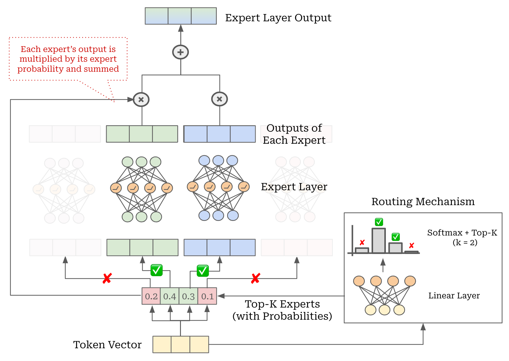
Computing expert layer output. Once we have used the routing mechanism to determine the set of active experts for a given token, we can compute the final output for this expert layer as follows:

1. Send the tokens to their active experts.

2. Compute the output of the active experts for these tokens.

3. Take a weighted average of expert outputs for each token, where the weights are simply the probabilities assigned to each active expert by the router.

This process is depicted for a single token in the figure above. Recent research on MoEs has also introduced the idea of “shared” experts, which are always active for all tokens. Shared experts slightly modify the routing logic, but the same core ideas outlined above still apply; see here for more details on this topic.

An implementation of a full expert layer is provided below, where we see these ideas applied in PyTorch. On line 49, we get the batches of data for each expert—and the associated expert probabilities for each token—from our router. We then pass these batches through our expert feed-forward networks (line 52) to get the output of each expert. Finally, we multiply each expert’s output by the associated probability in lines 54-58, thus forming the final output of the expert layer.

This file contains bidirectional Unicode text that may be interpreted or compiled differently than what appears below. To review, open the file in an editor that reveals hidden Unicode characters. Learn more about bidirectional Unicode characters

Show hidden characters

	"""
	Based upon ColossalAI OpenMoE
	"""
	from torch import nn
	class MOELayer(nn.Module):
	def __init__(
	self,
	d,
	n_exp = 8,
	top_k = 2,
	use_noisy_top_k = True,
	capacity_factor = 1.25,
	bias=False,
	dropout=0.2,
	):
	"""
	Arguments:
	d: size of embedding dimension
	n_exp: the number of experts to create in the expert layer
	top_k: the number of active experts for each token
	use_noisy_top_k: whether to add noise when computing expert output
	capacity_factor: used to compute expert capacity
	bias: whether or not to use bias in linear layers
	dropout: probability of dropout
	"""
	super().__init__()
	self.router = Router( # (noisy) top k router
	d=d,
	n_exp=n_exp,
	top_k=top_k,
	use_noisy_top_k=use_noisy_top_k,
	capacity_factor=capacity_factor,
	)
	self.experts = MLPExperts( # group of MLPs (experts)
	d=d,
	n_exp=n_exp,
	bias=bias,
	dropout=dropout,
	)
	def forward(self, x: torch.Tensor):
	B, C, d = x.size() # track original shape of input
	num_tokens = (B * C)
	# pass each token through the router
	exp_weight, exp_mask, exp_batches = self.router(x)
	# compute expert output
	exp_out = self.experts(exp_batches) # [n_exp, exp_capacity, d]
	# aggregate expert outputs based on router weights
	# eq (2) on page 4 of ST-MoE (https://arxiv.org/abs/2202.08906)
	exp_weight = exp_weight.view(num_tokens, -1) # [B * C, n_exp * exp_capacity]
	exp_out = exp_out.view(-1, d) # [n_exp * exp_capacity, d]
	output = exp_weight @ exp_out # [B * C, d]
	# resize output before return
	return output.view(B, T, d)

view raw expert_layer.py hosted with ❤ by GitHub

MoE in PyTorch. Now, we can modify the decoder-only transformer block to optionally use an expert layer in place of the usual feed-forward layer. This is accomplished in the code below, where we do a drop-in replacement of our MLP module with the new MoELayer, forming an MoEBlock.

This file contains bidirectional Unicode text that may be interpreted or compiled differently than what appears below. To review, open the file in an editor that reveals hidden Unicode characters. Learn more about bidirectional Unicode characters

Show hidden characters

	from torch import nn
	class MoEBlock(nn.Module):
	def __init__(
	self,
	d,
	H,
	C,
	n_exp,
	top_k,
	use_noisy_top_k = True,
	capacity_factor = 1.25,
	bias = False,
	dropout = 0.2,
	):
	"""
	Arguments:
	d: size of embedding dimension
	H: number of attention heads
	C: maximum length of input sequences (in tokens)
	n_exp: the number of experts to create in the expert layer
	top_k: the number of active experts for each token
	use_noisy_top_k: whether to add noise when computing expert output
	capacity_factor: used to compute expert capacity
	bias: whether or not to use bias in linear layers
	dropout: probability of dropout
	"""
	super().__init__()
	self.ln_1 = nn.LayerNorm(d)
	self.attn = CausalSelfAttention(d, H, T, bias, dropout)
	self.ln_2 = nn.LayerNorm(d)
	self.mlp = MOELayer(
	d,
	n_exp,
	top_k,
	use_noisy_top_k,
	capacity_factor,
	bias,
	dropout,
	)
	def forward(self, x):
	x = x + self.attn(self.ln_1(x))
	x = x + self.mlp(self.ln_2(x))
	return x

view raw moe_block.py hosted with ❤ by GitHub

From here, the final implementation of our MoE architecture exactly matches the decoder-only transformer (GPT) implementation from before. The only change is that we replace every P-th Block with an MoEBlock. We will avoid explicitly writing out this implementation here, as the code is identical to the GPT model defined before, aside from the addition of interleaved MoE blocks.

Pretraining nanoMoE from Scratch

Now that we understanding how MoEs work, let’s pretrain an LLM from scratch using this architecture. A full implementation of an MoE-based LLM is present in the repository below. This implementation—called nanoMoE—is based upon Andrej Karpathy’s nanoGPT repository. However, the original GPT architecture has been modified to use an MoE-based decoder-only transformer architecture.

The nanoMoE repository reuses code for all of the MoE components that we have seen so far in this post. The key components of this implementation are:

• Model implementation: see the GPT model definition, where the ability to construct an MoE model has been added. [link]

• Training: all training code is present in a single file and has not been meaningfully modified from the original nanoGPT code. [link]

• Dataset: nanoMoE is pretrained on a 25B token subset¹² of the OpenWebText dataset (same as nanoGPT but with fewer tokens). [link]

• Configuration: the final training configuration used to pretrain nanoMoE, which we will explain in the next section, can be found here.

In this section, we will further outline the best practices that were discovered for successfully pretraining nanoMoE, go over the results of pretraining, and outline the optimal pretraining setup that was discovered for this mid-size MoE model.

Best Practices for Training MoEs

“Despite several notable successes of MoE, widespread adoption has been hindered by complexity, communication costs and training instability.” - from [6]

Although MoEs were proposed a long time ago, their popularity has increased drastically for LLM research only recently. For years, the main impediment to the adoption of MoEs was their difficulty of use. Relative to dense models, MoEs are more complex and generally prone to instability during training.

Why are MoEs unstable? As we have seen, MoE-based LLMs only make slight modifications to the decoder-only transformer architecture. With this in mind, we might wonder: What exactly in the MoE architecture causes difficulty during training? Why is the training of an MoE less stable compared to a standard LLM?

Divergence during nanoMoE pretraining

There are two main issues that occur when training an MoE:

1. Routing collapse: the model converges to utilizing the same expert(s) over and over again.

2. Numerical instability: the MoE may experience round-off errors, especially in the router (i.e., due to its use of exponentials in the softmax)¹³.

These issues lead to training instability, meaning that the model’s loss may simply diverge during the training process; see above for a concrete example from training nanoMoE. When this happens, we need to stop the training process and restart from a saved checkpoint, which is time consuming and inefficient (i.e., lots of idle GPU time!). Ideally, we want a stable training process that avoids these instabilities. So, let’s cover best practices for improving MoE training stability.

Auxiliary losses. As discussed previously, we do not have to choose between auxiliary losses when training an MoE. Instead, we can just combine multiple auxiliary losses into a single loss function. In the case of nanoMoE, we use both the standard auxiliary load balancing loss and the router z-loss during training. Using the correct auxiliary losses improves training stability by enabling uniform usage of experts and avoiding routing collapse during training.

Training precision. When training an LLM, it usually makes sense to use mixed precision training, which converts some components of the model to run in a lower float16 or bfloat16 precision format instead of full float32 precision. This functionality is supported automatically in PyTorch via the automatic mixed precision (AMP) module and can significantly reduce training costs without deteriorating model performance. In other words, this is a “free” pretraining speedup that we can easily enable with minimal code changes.

“Compared with the BF16 baseline, the relative loss error of our FP8-training model remains consistently below 0.25%, a level well within the acceptable range of training randomness.” - from [8]

Mixed precision has been used for some time, but researchers have more recently explored methods for reducing LLM training precision even further—lower than 16-bits. For example, DeepSeek-v3 [8] is trained using 8-bit precision. However, maintaining the same level of model quality becomes more difficult as training precision is reduced. Implementing large-scale LLM training with FP8 precision requires novel and complex quantization techniques. Otherwise, training an LLM at such low precision may negatively impact the model’s performance.

with torch.amp.autocast(device_type='cuda', enabled=False):
    # AMP is disabled for code in this block!
    <router code goes here>

Why is this relevant to MoEs? As we mentioned before, the routing mechanism within an MoE is prone to numerical instability. Computing the router’s output in lower precision makes this problem even worse! This issue is explicitly outlined in [6], where authors find that low precision training leads to large round-off errors in the router. To solve this issue, we must run the router in full (float32) precision even when training with AMP, which can be achieved by simply disabling AMP in the MoE’s routing mechanism; see above.

Weight initialization. Traditionally, one of the biggest factors for stable training of large neural networks has been using the correct weight initialization strategy; e.g., Glorot or He initialization. These techniques—along with strategies like batch normalization—unlocked the ability to train incredibly deep neural networks, which was quite difficult before. For LLMs, we usually adopt these same weight initialization strategies. However, authors in [6] recommend adopting a slightly modified weight initialization scheme that is specifically designed for MoEs.

# linear layers have flipped dimensions ([out_dim, in_dim]) in torch
w_fan_in = module.weight.shape[-1]
w_std = (scale / w_fan_in) ** 0.5
torch.nn.init.trunc_normal_(
    module.weight,
    mean=0.0,
    std=w_std,
    a=-2*w_std,
    b=2*w_std,
)

This weight initialization strategy samples weights from a truncated normal distribution with a mean of zero (µ = 0) and standard deviation given by σ = SQRT(s/n), where s is a scale hyperparameter and n is the size of the input to the layer being initialized (i.e., fan-in strategy). Authors in [6] also recommend using a reduced scale hyperparameter of s = 0.1 to “improve quality and reduce the likelihood of destabilized training”. An implementation of this modified weight initialization strategy in PyTorch is provided above.

MoE finetuning. We will only focus on pretraining nanoMoE in this overview. However, we should also be aware that MoEs can be more difficult to finetune compared to standard dense models. In particular, MoEs are prone to overfitting due to the fact that they have so many parameters. These large models are great for pretraining over massive datasets, but they can overfit when finetuned over a small amount of data. We should be aware of this issue and try our best to prevent overfitting when finetuning MoEs (e.g., via a higher dropout ratio). We leave the exploration of finetuning nanoMoE—and preventing overfitting—as future work.

nanoMoE Pretraining Experiments

Now that we understand the different tricks that we can use to train MoEs in a stable fashion, let’s test them out in real life by pretraining nanoMoE from scratch. To test these commands yourself, you will need access to one or more GPUs. For the experiments presented here, I used two RTX 3090 GPUs on my personal workstation. These are commodity GPUs—they do not have much memory (only 24 Gb). The pretraining settings have been scaled down accordingly, allowing everything to fit in GPU memory and run completely in less than a week.

General pretraining settings. The final configuration used for pretraining is here and has the following settings:

• Model architecture: six layers (or blocks), six attention heads per self-attention layer, d = 368, N = 8 (total experts), K = 2 (active experts), P = 2 (every other layer uses an MoE block).

• Expert capacity: capacity factor of 1.25 for training and 2.0 for evaluation.

• Auxiliary losses: we use both the load balancing auxiliary loss (scaling factor of 0.01) and the router z-loss (scaling factor of 0.001).

• Precision: we use automatic mixed precision (bfloat16) for training but the router always uses full (float32) precision.

• Learning rate: we adopt a standard LLM learning rate strategy—linear warmup from 6e-5 to 6e-4 at the start of training, followed by cosine decay to 6e-5.

• Weight initialization: we use the weight initialization scheme proposed in [6] to improve MoE training stability.

Pretraining dataset. Similarly to nanoGPT, we use the OpenWebText dataset for pretraining nanoMoE. The pretraining process is scaled down to ~25 billion total tokens—around 10% of the tokens used for pretraining nanoGPT. This smaller dataset allows pretraining to complete in roughly 5 days on two 3090 GPUs. However, we can easily scale this up to a full pretraining run by obtaining a better GPU setup (e.g., 8×A100 GPUs) and setting max_iters = 600,000 (instead of 50,000).

Stability experiments. To test the impact of different settings on nanoMoE’s training stability, we perform five different experiments. First, we pretrain a baseline nanoMoE model using no auxiliary losses or best practices, which leads to poor load balancing and instability. Then, we enable several improvements one-by-one to observe their impact on pretraining stability:

1. Auxiliary load balancing loss.

2. Router z-loss.

3. Full precision in the router.

4. Improved weight initialization scheme.

The results of these five experiments are shown in the figure below. As we can see, each improvement to the pretraining process yields a slight improvement in training stability—the divergence in pretraining comes a little bit later in the training process. When we enable all of the improvements together, the model actually completes the entire training process without any issues! We can clearly see here that the ideas discussed tangibly impact nanoMoE’s training stability.

Testing different stability techniques for nanoMoE

For those who are interested, I would encourage you to try these ideas out yourself! Just tweak the training configuration and execute the pretraining process using the command shown below. This command assumes that you are running pretraining on a single node with one or more GPUs available.

torchrun --standalone --nproc_per_node=<number of GPUs> train.py <path to config; e.g., config/train_nano_moe.py>

Further Learning for Mixture-of-Experts

In this overview, we have gained an in-depth understanding of how Mixture-of-Experts (MoE)-based LLMs operate by beginning with a standard decoder-only transformer architecture and modifying it to use an MoE architecture. Then, we applied these ideas by pretraining a mid-size MoE-based LLM, called nanoMoE, from scratch on the OpenWebText dataset. Although MoEs are considered to be more difficult to train than standard LLMs, we see in our experiments how ideas like auxiliary losses, mixed precision, better weight initialization and more can be applied to train MoEs successfully (i.e., without any instabilities)!

Although nanoMoE is a great learning tool, most practical implementations of MoEs will be more complex than this. To learn about how MoEs are actually used in LLM research, we should look at production-grade MoE frameworks for efficient training and inference (e.g., OpenMoE [9] or Megablocks [10]), as well as recent publications on the topic of MoEs; e.g., Mixtral, DeepSeek-v3, or DBRX.

New to the newsletter?

Hi! I’m Cameron R. Wolfe, Deep Learning Ph.D. and Research Scientist at Netflix. This is the Deep (Learning) Focus newsletter, where I help readers understand important topics in AI research. If you like the newsletter, please subscribe, share it, or follow me on X and LinkedIn!

Bibliography

[1] Vaswani, Ashish, et al. "Attention is all you need." Advances in neural information processing systems 30 (2017).

[2] Sennrich, Rico, Barry Haddow, and Alexandra Birch. "Neural machine translation of rare words with subword units." arXiv preprint arXiv:1508.07909 (2015).

[3] Shazeer, Noam. "Glu variants improve transformer." arXiv preprint arXiv:2002.05202 (2020).

[4] He, Kaiming, et al. "Deep residual learning for image recognition." Proceedings of the IEEE conference on computer vision and pattern recognition. 2016.

[5] Zoph, Barret, et al. "St-moe: Designing stable and transferable sparse expert models." arXiv preprint arXiv:2202.08906 (2022).

[6] Fedus, William, Barret Zoph, and Noam Shazeer. "Switch transformers: Scaling to trillion parameter models with simple and efficient sparsity." Journal of Machine Learning Research 23.120 (2022): 1-39.

[7] Shazeer, Noam, et al. "Outrageously large neural networks: The sparsely-gated mixture-of-experts layer." arXiv preprint arXiv:1701.06538 (2017).

[8] Liu, Aixin, et al. "Deepseek-v3 technical report." arXiv preprint arXiv:2412.19437 (2024).

[9] Xue, Fuzhao, et al. "Openmoe: An early effort on open mixture-of-experts language models." arXiv preprint arXiv:2402.01739 (2024).

[10] Gale, Trevor, et al. "Megablocks: Efficient sparse training with mixture-of-experts." Proceedings of Machine Learning and Systems 5 (2023): 288-304.

1. This architecture is not “new” per se. It has been around for a very long time. But, it’s adoption in large-scale LLM applications is more recent.

2. The decoder is slightly different because we remove the cross-attention layer that is used in the decoder for the full encoder-decoder model.

3. An explanation of basic positional encodings (or embeddings) for transformers can be found here. However, most modern LLMs use rotary positional embeddings (RoPE) in place of this basic position encoding scheme from [1].

4. Our implementation here also performs attention dropout, where we randomly drop certain attention scores during training for regularization purposes.

5. The word “pointwise” indicates that the same operation is applied to every token vector in the sequence. In this case, we individually pass every token vector in the sequence through the same feed-forward neural network with the same weights.

6. We use a pre-normalization structure, where normalization is applied to the input of each layer. The original transformer [1] used a post-normalization structure, but later analysis showed that pre-normalization is favorable.

7. To apply a residual connection within a neural network layer, the input and output dimension of that layer must be the same. If the dimensions are not the same, we can still apply a residual connection by just linearly projecting the input.

8. See [5] and [6] for more details and experiments on tuning the capacity factor.

9. The details are not super important here—this is just an implementation complexity that is introduced to vectorize the operations of the router. However, this is a great coding exercise in PyTorch for those who are interested in understanding!

10. This quantity is predicted by our routing algorithm and is, therefore, differentiable. So, the loss function as a whole is differentiable even though the fraction of tokens sent to each expert is not itself a differentiable quantity.

11. We also multiply the result of the operation by N (the total number of experts), which ensures that the loss stays constant as the value of N increases.

12. This number of tokens was selected such that the full pretraining run can be completed in ~5 days on a 2× RTX 3090 GPU setup.

13. Although softmax transformations are a pretty common operation, we should note that standard decoder-only transformers do NOT have these exponentials anywhere within their architecture!