Model Merging: A Survey
From modern LLM applications to the early days of machine learning research...
To improve the performance of a machine learning model, we can train several models independently and average their predictions at inference time to form an ensemble. Ensembling has been used for decades in machine learning, but this approach comes with the downside of increased inference costs—we must compute the output of several models!1 To avoid this issue, researchers have explored alternative techniques for combining models. These explorations eventually led to the popularization of weight-space ensembles, which average the weights of the models in an ensemble—forming a single, merged model—instead of averaging their predictions. This technique was found to perform quite well, matching or exceeding the performance of vanilla, output-space ensembles in many cases.
“We unveil that Language Models (LMs) can acquire new capabilities by assimilating parameters from homologous models without retraining or GPUs.” - from [3]
Today, model merging is a popular research topic, but this idea is not new whatsoever—we can trace it all the way back to the 1990s [7]! In the deep learning era2, techniques related to model merging have repeatedly appeared in research topics like mode connectivity, generalization, continual learning and more. In the last few years especially, the level of interest in model merging has exploded due to its effectiveness in applications with large language models (LLMs). We have seen model merging used to combine the capabilities of several foundation models, inject new skills into a model, or even improve the alignment process. In this overview, we will take a deep look at all of this research, starting from the beginning and working our way up to modern applications with LLMs.
Foundations and Background Information
Before diving into recent research on model merging, we will take a look at the early work in this space. Additionally, we will explore a few different, but related, research topics that from the basis of model merging. By better understanding these techniques and their origins, we will gain a more nuanced perspective on model merging techniques, allowing us to more deeply understand the core ideas in this space, where they come from, and why they work so well.
The Origins of Model Merging
Model merging is a popular research topic as of late, but the history of this technique is quite extensive, dating all the way back to the mid 1990s! Authors in [7] observe that practitioners oftentimes train several machine learning models for a given problem, where each model differs in its architecture, training data composition, and/or hyperparameter settings. These models are then used to form an ensemble by combining the outputs of the various models, either by taking an average of outputs or learning weights to be associated with each model’s output.
“We … propose that under certain conditions one can average model parameters directly instead of retaining all networks and combine their outputs.” - from [7]
In the case of (simple) neural networks, we see in [7] that one can average model parameters directly instead of averaging model outputs. This approach yields similar performance to taking an average of each model’s output, while saving on both storage and compute costs. Most of the work we will see in this overview came long after [7], but this work served as a catalyst for model merging research, which—as we will see—became a fruitful and important topic of investigation.
(Linear) Mode Connectivity
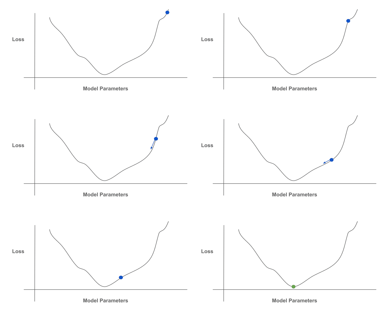
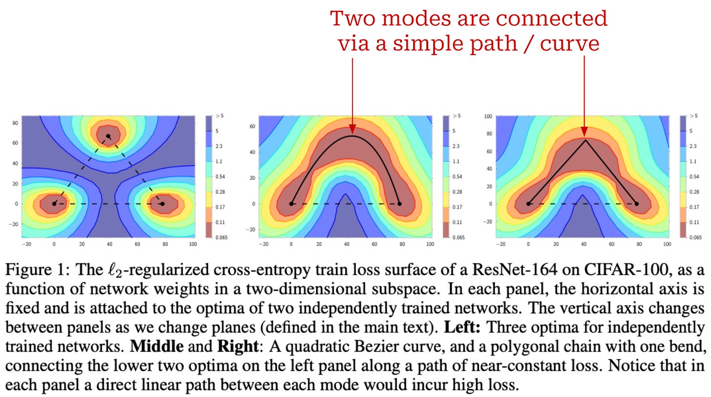
When we first learn about training a machine learning model via gradient-based optimization techniques (e.g., stochastic gradient descent), we are typically shown a very simple, 1D view of a loss function being minimized; see above. In reality, the loss landscape of a neural network is non-convex and chaotic, as shown in the image below. However, there are some predictable properties and behaviors of these loss landscapes that we have observed empirically, which make them a little bit less intimidating. One of these interesting properties is mode connectivity.

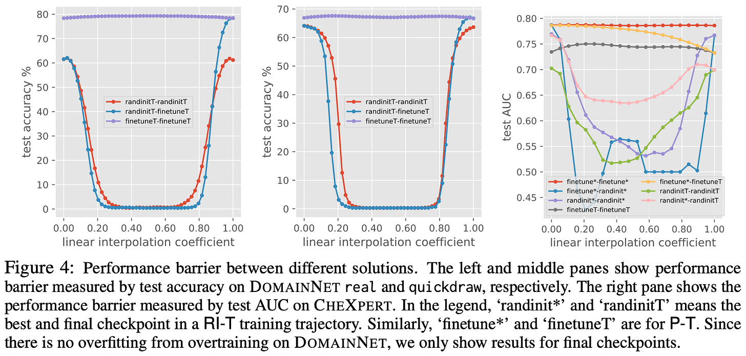
Mode connectivity is an idea that was originally observed and coined in [11]. The training dynamics of neural networks are complex, as we see in the visualization above. For this reason, we might think that two independently-trained neural networks3 would end up in completely different regions of the optimization landscape. In [11], we learn that this is not always true—the training trajectory of a neural network becomes relatively predictable after a certain number of iterations.
“We show that the optima of these complex loss functions are in fact connected by simple curves over which training and test accuracy are nearly constant.” - from [11]
In particular, authors in [11] observe that the weights of neural networks that are trained independently can be connected together in the loss landscape via a path of constant training and test accuracy4, which can be discovered via their novel training procedure. Interestingly, these “modes” (i.e., the location of the trained network’s weights in the loss landscape) are usually connected by simple curves, as shown within the figure below. This idea was coined mode connectivity due to our ability to connect the modes of these networks via simple paths of constant performance. This property was shown in [11] to hold for numerous computer vision architectures (primarily ResNets) trained on several popular datasets.
Linear mode connectivity is a more specific case of mode connectivity that is observed and analyzed in [12]. Authors in this paper study and compare the properties of vision models trained with different random noise. In particular, the data ordering and augmentation adopted during training, which is referred to as SGD noise in [12], is varied. Then, the mode connectivity between the resulting models obtained via training with varying levels of SGD noise is studied.
To check if two networks are linearly mode connected, we just (linearly) interpolate between their weights and check that the training and test loss of models obtained along this path of linear interpolation is constant. Verifying linear mode connectivity is much simpler compared to mode connectivity in general, as we just have to check a linear path between the models’ weights, instead of using a more complex training algorithm to search for an arbitrary mode connected path. Going further, authors in [12] extend this analysis by only varying SGD noise after k training iterations have been performed; see above.
We learn in [12] that neural networks become stable to SGD noise—meaning that models trained with varying levels of SGD noise are still linearly mode connected after training—very early in training. After a certain (reasonable) amount of training, all networks obtained from the same base model are linearly mode connected. As we will see, this finding is highly related to model merging, as we typically merge models by averaging or interpolating their weights. As such, linear mode connectivity provides empirical intuition for why such interpolated weights perform well!
To make this idea a bit more specific, later work in [13] shows models that are finetuned from the same pretrained weights end up in the same basin (or region) of the loss landscape. In other words, independently finetuned models that start from the same base model end up close to each other in the parameter space—this observation has deep connections to research on critical learning periods. This region of the loss landscape contains several viable model parameters settings that can be discovered, which provides further explanation for the effectiveness of merging and interpolation techniques that will be explored throughout this overview.
Mode connectivity and LLMs. In [14], authors perform a similar analysis of linear mode connectivity for LLMs. From these experiments, we learn that finetuned LLMs tend to be linearly mode connected, but these models must be finetuned starting from the same pretrained weights for mode connectivity to hold! As shown above, numerous interpolation strategies are explored in [14] with GPT-style LLMs—GPT-2 in particular. This work successfully demonstrates the applicability of linear mode connectivity to modern language models.
Pruning and Sparsity for Language Models
Throughout this overview, we will study several works that explain the mechanisms that make model merging possible. At a high level, one important reason that model merging tends to be so effective is that large neural networks—and LLMs in particular—usually exhibit high levels of sparsity. The weights and activations within these models have a few important values, while other values are either redundant or not impactful; see above. As a result, we can eliminate a large ratio of model parameters via techniques like pruning without meaningfully impacting performance, as well as merge parameters without a high likelihood of two important weights or activations conflicting with each other.
Neural network pruning starts with a large neural network and aims to derive from this larger network a smaller network with comparable performance. To do this, we usually follow a multi-step process (shown above) of:
Training the model to convergence.
Pruning the model’s weights (e.g., via a heuristic like removing the lowest-magnitude weights in each layer).
(Optionally) rewinding the model’s remaining weights to their original values.
Training the subnetwork (i.e., the pruned model) to convergence.
We can repeatedly apply steps two through four to derive an iterative pruning strategy, which allows higher performance to be maintained by slowly removing weights from the model instead of pruning many weights at the same time. By following this strategy, we can derive incredibly small networks that achieve performance that is comparable to—or even better than—the larger models from which they are derived. For this reason, pruning became a popular research topic in the late 2010’s and continues to be an active direction of research even today.
“We articulate the lottery ticket hypothesis: dense, randomly-initialized, feed-forward networks contain subnetworks (winning tickets) that—when trained in isolation—reach test accuracy comparable to the original network in a similar number of iterations.” - from [16]
In a prior overview5, we learned about the topic of neural network pruning in great depth; see here. For those who want to learn more, I have also listed my favorite pruning papers below:
Learning Structured Sparsity in Deep Neural Networks: this paper is the first to explore pruning via the L1-norm heuristic (i.e., removing low magnitude weights), which is the most commonly-used pruning strategy.
Pruning Filters for Efficient ConvNets: this paper shows significant reductions in the compute cost of a neural network can be achieved without a reduction in performance by removing filters with low L1-Norm from a model’s layers.
Rethinking the Value of Network Pruning: this work performs an extensive empirical analysis of different pruning techniques and settings to determine best practices for obtaining high-performing subnetworks.
The Lottery Ticket Hypothesis: this paper discovers and analyzes the lottery ticket hypothesis (LTH), which shows that high-performing subnetworks exist within the randomly-initialized weights of a neural network.
Despite becoming a very popular research topic in recent years, the idea of pruning has deep roots in early research on neural networks. Some of the first works to explore this idea were written in the early 1990s [17, 18]; see below.
Pruning in the age of LLMs. More recently, research on neural network pruning has been modernized in the age of LLMs. In [19], authors propose a pruning algorithm, called SparseGPT, that can be used to prune GPT-style language models—using an unstructured approach—to over 50% sparsity in one shot, meaning that no retraining is required after pruning. Eliminating retraining from the pruning procedure reduces compute costs significantly. The SparseGPT algorithm, which is shown below, operates by reducing the pruning process into a series of sparse regression problems that can be approximated efficiently.
Shortly after, authors in [19] performed analysis showing that magnitude-based pruning—a popular and widely-used technique for pruning—works poorly for LLMs. Although SparseGPT improves upon this technique, authors mention that this pruning algorithm takes around 4-5 hours to execute for a ~100B parameter LLM when running on a single GPU. In other words, the SparseGPT algorithm is still computationally expensive even if it does not require retraining to be performed.
“Considering the past success of magnitude pruning on smaller networks, this result suggests that LLMs, despite having 100 to 1000 times more parameters, are substantially more difficult to prune directly.” - from [20]
As a solution, Wanda (pruning by Weights AND Activations)—a very simple pruning approach for LLMs—is proposed and analyzed in [20]. This approach determines which weights to prune by multiplying each of the model’s weights by their corresponding input activations on a per-output basis; see below for the exact formulation. Similar to SparseGPT, this technique requires no retraining. Additionally, Wanda is more efficient as a whole, and we can achieve higher levels of sparsity without damaging the performance of the pruned model. From this work, we learn that effectively pruning LLMs is difficult, but possible.
Although the technique used for pruning within Wanda might seem random, the algorithm in [20] is actually inspired by the recent observation that LLMs tend to have a small number of very high magnitude activations within each of their hidden layers. Interestingly, these high magnitude features (or outliers) seem to be an emergent property of larger models (i.e., ~7B parameters and beyond).
“At around 6.7B parameters, a phase shift occurs, and all transformer layers and 75% of all sequence dimensions are affected by extreme magnitude features.” - from [21]
This property was first observed in the quantization context [21], where authors develop a more performant 8-bit quantization technique for LLM inference by adopting tricks to property deal with these outliers features; see below.
However, another work [15] also explores this property in depth, finding that these massive activations exist across a wide variety of different models and training settings. Put simply, work in [15] and [21] shows us that LLMs tend to have incredibly sparse activations that can be exploited for better pruning.
Why does this matter? Although pruning and model merging are separate topics, they are highly related due to their joint dependence upon the same fundamental idea—sparsity. Understanding pruning algorithms and related research is highly beneficial when learning about model merging, especially given that pruning is such a comprehensively-studied topic with an abundance of great ideas.
Early Work on Model Merging
Now that we understand the fundamental concepts that underlie the concept of model merging, we will look at a collection of notable papers that initially explored the concept of model merging for deep neural networks. Most of these papers were published prior to the popularization of LLMs, but many of the techniques are repurposed in the research we see on model merging today.
Model soups: averaging weights of multiple fine-tuned models improves accuracy without increasing inference time [5]
When we finetune a pretrained model on some downstream task, the best training hyperparameters to use are oftentimes unknown. As a result, we usually i) run several training trials with different hyperparameters, ii) select the model that performs best on some held-out validation set, and iii) discard the remaining models. Instead of discarding remaining models, we could form an ensemble of these models, which usually improves performance [6]. But, this approach drastically increases inference costs. In [5], authors explore an alternative strategy—merging the weights of these models—that can have the best of both worlds!
“Model soups can approach the performance of ensembling, with no additional computational cost or memory relative to a single model during inference.” - from [5]
Model soups. The idea proposed in [5] is very simple—we finetune several identical models with different hyperparameter settings and merge their weights. Although we usually discard all but the best model when performing hyperparameter tuning, this approach is inspired by work on model ensembling that shows the benefit of averaging the predictions of these models. There are a few different ways we can merge the models’ weights! The following techniques are considered in [5]:
Average: just take a uniform average of models’ weights.
Greedy: select only models with performance above some threshold (e.g., average model performance) and take the average of selected models’ weights.
The resulting merged model is referred to as a “model soup”. Authors in [5] also propose a more sophisticated technique for learning optimal merging coefficients between model weights. However, this approach requires all models to be loaded into memory at the same time, which is impractical.
When comparing average and greedy merging, we see in [5] that better performance is generally achieved with greedy merging. The issue with average merging is that certain hyperparameter settings may lead a subset of resulting models to perform poorly compared to others. Greedy merging removes these models from consideration via a simple performance filter; see above. More specifically, greedy soups are constructed by sequentially adding each model to the soup only if performance on a held-out validation set is improved. The list of considered model is sorted in decreasing order of validation set performance beforehand, ensuring that the greedy soups is no worse than the best individual model.
How well does this work? Experiments in [5] largely consider the task of image classification on ImageNet, but a variety of models are considered, including CLIP, ALIGN, BASIC, and several vision transformer (ViT) variants. These models are all pretrained on a separate large-scale dataset (e.g., WIT or JFT-3B), finetuned on ImageNet, and evaluated on ImageNet6.
The high level results of these experiments are outlined in the table above. For any number of models, the greedy soup consistently outperforms the best single model of any hyperparameter sweep, as well as nearly matches the performance of model ensembles in most cases. Unlike an ensemble, however, the model soup incurs no additional inference or memory cost relative to a single model!
Authors in [5] even reach new state-of-the-art performance on ImageNet, achieving a test accuracy of 90.94%7 with a soup of ViT-G models. Model soups also perform better in the zero-shot regime and on new tasks that go beyond the distribution of the ImageNet test set. Additionally, model soups are found to yield useful results on text classification tasks with transformers; see above.
Why does this work? Authors in [5] provide extensive analysis to motivate and explain the effectiveness of model soups. Much of this analysis draws parallels to prior research on linear mode connectivity. As shown in the figure above, finetuned models tend to lie within a similar basin of the loss landscape, meaning that the loss is relatively stable—and might even decrease—when we interpolate between the weights of these finetuned models! The best performing model is not any of the individual finetuned models. Rather, it lies somewhere in the loss landscape between all of these models. So, interpolating between these models via a model soup allows us to discover higher-performing models!
Model Ratatouille [36] is an interesting extension to model soups that aims to repurpose the large variety of finetuned foundation models that are available online. Our goal is to finetune a model on a downstream task. Instead of directly finetuning a single model, however, we do the following (shown above):
Obtain several openly-available models that have been finetuned on different auxiliary tasks.
Finetune each of these models separately on our downstream task.
Merge the weights (via an average) of all finetuned models.
We see in [36] that such a technique outperforms prior merging techniques, demonstrating that the extra information learned by these models when finetuned on diverse auxiliary tasks is useful for forming model soups.
Robust fine-tuning of zero-shot models [8]
“Can zero-shot [foundation] models be fine-tuned without reducing accuracy under distribution shift?” - from [8]
When we train a foundation model, we would like for this model to work well across a broad distribution of data. The advent of self-supervised pretraining has largely solved this problem—pretrained LLMs can solve a wide variety of problems in a zero-shot manner due to their sizable knowledge base that is derived from the massive text corpus on which the model is pretrained. Still, we can improve the performance of a pretrained model on a particular target domain by finetuning the model on a targeted set of data from that domain8; see below.
Despite the utility of finetuning, there are downsides of which we should be aware! Finetuning a pretrained model on a domain-specific dataset:
Improves the model’s performance on data from that particular domain.
Degrades the model’s performance on data beyond that particular domain.
Put simply, finetuning makes the model less generic, which can degrade its performance on data that is different from the finetuning dataset. In [8], authors try to mitigate this issue by adopting a simple model merging approach.
Finetuning and robustness. The negative impact of finetuning on the robustness of a pretrained model makes sense intuitively. Finetuning a pretrained model specializes this model to the properties of data from the target domain, which comes at the cost of model performance in a broader sense. Although the impact of finetuning on model robustness makes sense intuitively, authors in [8] analyze this relationship in more detail. In particular, several interesting findings regarding the impact of finetuning on model performance are outlined:
The model’s performance improves on the target distribution.
The model’s performance degrades under various distribution shifts (i.e., data that goes beyond the target distribution).
Hyperparameter settings have a very large impact on robustness.
More “aggressive” finetuning (e.g., using a larger learning rate) exacerbates these findings—target domain performance improves more and performance is even worse under distribution shifts.
To measure accuracy under distribution shifts, we can simply adopt existing datasets from out-of-distribution (OOD) generalization research. For example, the ImageNet dataset has numerous alternative test sets that can be used to study several kinds of distribution shifts; see below for a few examples.
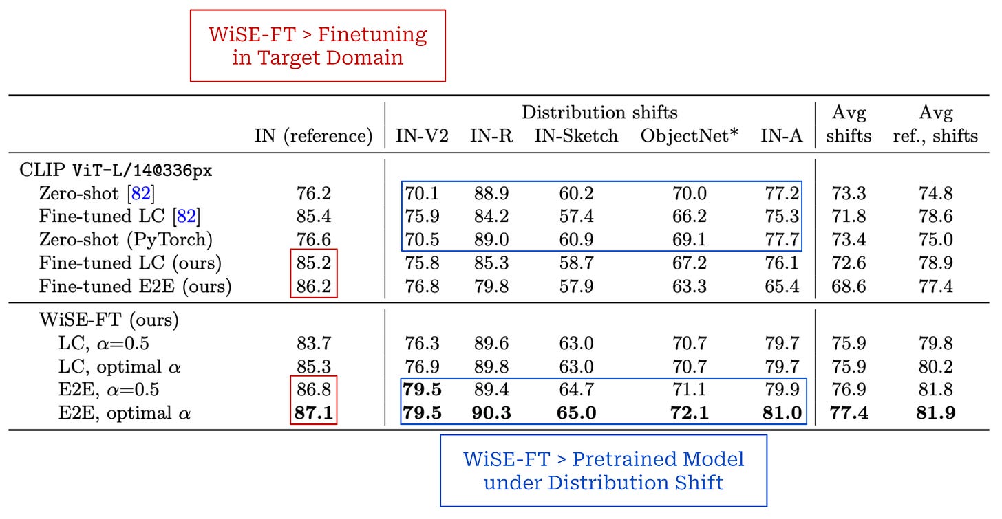
Weight-Space Ensembles for Fine-Tuning (WiSE-FT). The technique proposed in [8] is simple. We i) start with a pretrained model, ii) finetune the model on a target dataset, and iii) interpolate between the weights of the pretrained and finetuned models; see below. Although we can arbitrarily interpolate between the weights of the pretrained and finetuned models, we see in [8] that simply taking an average of these weights works well in most cases.
Extending upon research on linear mode connectivity, authors in [8] observe that finetuned models are typically mode connected to their associated base model. More generally, we learn that models sharing a large part of their training trajectory—such as a pretrained model and any finetuned models derived from this pretrained model—tend to be mode connected, which allows us to merge these models without causing a catastrophic impact to performance.
Does this work well? The impact of WiSE-FT is mostly studied using pretrained CLIP models on the ImageNet dataset, where we see that merging pretrained and finetuned models yields a happy medium between the performance of both models. The results of the analysis in [8] are summarized in the figure above.
In short, WiSE-FT yields the following benefits compared to a model obtained via standard finetuning (see table above for more details):
Improved accuracy under distribution shifts.
Comparable (or improved) accuracy in the target domain.
We also see that WiSE-FT can mitigate the sensitivity of model robustness to hyperparameter settings—we can recover the performance of the best hyperparameter setting in nearly all cases by just changing the interpolation coefficient9. WiSE-FT also has no added computational costs during finetuning or inference.
Why does this work well? Beyond observing the performance benefits of WiSE-FT, authors dig a bit deeper into the mechanics of this technique by studying the relationship between the predictions generated by the pretrained, finetuned, and merged models. Interestingly, we see from this analysis that the finetuned model frequently overrides the predictions of the pretrained model when evaluating on in-domain data that is similar to the finetuning dataset. In contrast, predictions on out-of-distribution model are usually handled by the pretrained model! Put simply, the merged model naturally relies on the more appropriate model based upon the data (and task) being considered by a given input example.
“Overall, WiSE-FT is simple, universally applicable in the problems we studied, and can be implemented in a few lines of code. Hence we encourage its adoption for fine-tuning zero-shot models.” - from [8]
Implementation details. Given that WiSE-FT just takes a weighted average of model parameters, this technique is actually very easy to implement! An example using PyTorch syntax is provided in the algorithm below.
Further research. WiSE-FT is further analyzed in [42], where we see that this method also improves generalization via the “FalseFalseTrue” phenomenon. More specifically, WiSE-FT is observed to correct numerous cases where each model makes an incorrect prediction. The merged model is correct, but both of the source models are wrong! After analyzing this property theoretically, authors conclude that this property is largely due to impact of diverse feature sets on OOD generalization, thus providing (for the first time!) theoretical intuition for the ability of weight-space ensembles to outperform output-space ensembles.
An extension of WiSE-FT for LLMs, called an LM-Cocktail, is proposed in [49]. This approach merges finetuned language models with their pretrained base models, which mimics the strategy used in WiSE-FT. However, the technique is slightly more general, as additional models—such as those finetuned on data from other domains (i.e., peer models)—can also be included in the merge; see above.
Model Stock: All we need is just a few fine-tuned models [9]
Authors in [8] present a more recent extension of the model soups [5] and WiSE-FT [8] papers that aims to find a better tradeoff between:
The performance of the merged model.
The number of finetuned models we need to train (and merge).
Beginning with a pretrained model, the model soups technique proposed in [5] mandates that we perform several, independent finetuning runs, then take an average of the resulting models’ weights. Unfortunately, this technique typically requires that we finetune dozens of models, which is computationally expensive! Instead, WiSE-FT proposes finetuning a single model and interpolating between the weights of this model and the pretrained model, but performance is lacking.
“This strategy can be aptly coined Model Stock, highlighting its reliance on selecting a minimal number of models to draw a more optimized-averaged model.” - from [9]
To solve these issues, authors in [9] deeply analyze the geometric properties of finetuned weights relative to a pretrained model. This analysis allows them to devise an efficient merging strategy, called a model “stock”, that can achieve performance comparable to a model soup with only two finetuning runs, thus saving a massive amount of computation in terms of total training costs.
Geometric analysis. To arrive at this efficient merging strategy, we need to understand the properties of finetuned weights. What are model soups and WiSE-FT actually doing, and why do they work well? To answer these questions, authors in [9] finetune over 50 pretrained CLIP models and study how the finetuned weights relate to each other10, arriving at an interesting observation (depicted above):
All finetuned weights lie on a thin shell (or sphere) that is centered around a central point (i.e., the average of the finetuned weights), meaning the distance between finetuned weights and this center is (roughly) constant.
The center point lies at a different location in space relative to the pretrained weights, but these positions still satisfy predictable geometric properties.
This observation is empirically validated in [9] using several different finetuning setups, models, and datasets. Furthermore, we see from the analysis in [9] that these “central” weights—those lying at the center of all finetuned weights—consistently achieve optimal performance, exceeding the performance of all finetuned models and the pretrained model. This finding explains the utility of model soups—the model soup is an average of finetuned models and, therefore, an approximation of these central weights that are found to perform well.
“We uncover a strong link between the performance and proximity to the center of the weight space [and] introduce a method that approximates a center-close weight using only two finetuned models.” - from [9]
With this analysis in mind, WiSE-FT can be viewed as simply interpolating between the weights of a finetuned and pretrained model, which can be used to discover a point in space that is closer to the high-performing center; see below.
How can we use this? The analysis performed in [9] is incredibly thorough and interesting, but the details are intricate and beyond the scope of this post. I’d highly encourage the interested reader to check out sections two and three of the paper for the full details. The main question we want to answer here is: How can we practically leverage this information to create a better model merging technique?
The high-level answer is simple—we can use the geometric relationship between pretrained and finetuned model weights to efficiently approximate the center point. This approximation, which uses the properties discovered in [9] to directly solve for the center point, only requires two finetuned models to be generated; see above. The pretrained model serves as an “anchor point”, and we can approximate the center point by projecting it onto the plane formed by the weights of all three models.
There is a lot of fancy math here that can be a bit difficult to understand, but the practical result of this extensive analysis is just a different equation (shown above) for finding the best interpolation coefficient between finetuned weights! So, this approach is not actually that much different than WiSE-FT at the end of the day, we just i) train two finetuned models instead of one and ii) use a more intricate technique—based upon the geoemtric analysis in [9]—to optimally merge the models. However, WiSE-FT is more widely adopted in the literature due to its simplicity.
Empirical results. We see in [9] that closer proximity to the center point formed by the average of finetuned model weights—assuming the average is taken over a sufficiently large number of finetuned models—yields better performance, both on the target domain and under a distribution shift. Most experiments in [9] are performed using pretrained CLIP models that are finetuned on ImageNet, thus matching the experimental setup of WiSE-FT [8]. Model stocks with only two finetuned models are found to reach state-of-the-art performance on ImageNet and match the performance of model soups [5]—obtained using dozens of finetuned models—in this regime, thus yielding a significant reduction in training costs; see above. Interestingly, adding more models (i.e., three or four finetuned models) to a model stock does not yield a significant performance benefit; see below.
Weight Averaging Techniques
“We show that SGD generally converges to a point near the boundary of the wide flat region of optimal points. SWA is able to find a point centered in this region, often with slightly worse train loss but substantially better test error.” - from [22]
One common variant of model merging is simply taking an average of model weights at several points throughout the model’s training trajectory. More specifically, we i) record several checkpoints of the model’s weights throughout training, ii) take an average of the model’s weights at several checkpoints, and iii) use these averaged weights as our final model. This technique was originally proposed in [22]11 and is referred to as stochastic weight averaging (SWA); see below.
Compared to standard training (with stochastic gradient descent), SWA is shown in [22] to help the resulting model to generalize better. Plus, this technique is easy to implement and has no computational overhead, whereas alternative techniques (e.g., creating an ensemble of models) have significant increases in computation at inference time. We start with a pretrained network and apply SWA during the finetuning process, which ensures that the checkpoints are mode connected [13]. Numerous other weight averaging techniques have been explored as well:
DiWA [35] extends upon prior weight averaging techniques by improving the diversity of the models being averaged.
SWAD [41] extends SWA via a stochastic weight sampling strategy that finds flatter minima—with better generalization properties—in the loss landscape.
Fuse to Forget [43] studies the properties of knowledge within averaged models, finding that the resulting models tend to i) lose unshared knowledge and ii) have their shared knowledge enhanced.
Authors in [44] show that weight averaging can be used as a mechanism to mitigate catastrophic forgetting of old tasks when automatic speech recognition (ASR) models are adapted to new tasks.
We see in [45] that weight averaging is useful for merging learned policies—implemented as a “decision” transformer—for locomotion within reinforcement learning (RL), while [46] shows us that weight averaging is generally useful for improving training stability for RL with deep neural networks.
EMA of weights. Instead of taking an average over a finite and discrete number of model checkpoints, we can take an exponentially moving average (EMA) of model weights throughout the training process. This technique, which is an extension of SWA, was heavily adopted by vision models in the late 2010s (e.g., InceptionNet, EfficientNet, MnasNet, and more) but is not commonly covered in papers—it’s more of a practical implementation detail that can be found in the code repositories for these models. However, the concept of using EMA during training is mentioned in the original Adam optimizer paper [24]; see Section 7.2 here.
The idea of using models—or predictions—obtained via EMA as a target for self or semi-supervised learning has also been explored a lot [25, 26]; see above.
Extension to LLMs. In [27], authors explore an extension of SWA for LLM pretraining, leading to faster convergence and improved generalization. Two key observations inspire the proposed technique in [27]:
Models trained with a larger learning rate see more of a benefit from averaging model checkpoints along the training trajectory.
Averaging model trajectories that are further apart in the training process leads to larger gains.
Based on these findings, authors propose LAWA (LAtest Weight Averaging), which performs checkpoint averaging using a sliding window along the training trajectory of an LLM; see above for an illustration. LAWA simply maintains a first-in-first-out buffer of checkpoints sampled throughout the training process and computes an average over the k most recent checkpoints in this buffer. Checkpoints are inserted into the buffer with many training steps in between, ensuring that more distant checkpoints (i.e., those from the earlier phases of training) are included within the merging process; see below.
In [27], we see that LAWA outperforms conventional checkpoint averaging techniques like EMA and SWA in the language modeling domain, where larger learning rates are usually preferred. LLMs trained with LAWA converge faster and generalize better. The observed benefits of LAWA tend to improve as we add more training steps between the checkpoints that are sampled for averaging.
Model Merging for Large Language Models
Now that we have learned about early work on model merging, we will take a look at more recent techniques, such as task vectors, TIES, DARE, and more. Those who have tracked recent developments in LLM research are likely to have seen these techniques. Many of these algorithms are supported within popular open-source software for LLMs, such as the mergekit [54]. In this section, we will take a look at the most common algorithms used for merging LLMs, as well as learn about how model merging has transformed the LLM alignment process.
Editing Models with Task Arithmetic [1]
“With task arithmetic, practitioners can reuse or transfer knowledge from models they create, or from the multitude of publicly available models all without requiring access to data or additional training.” - from [1]
As practitioners, we usually solve tasks by i) starting with a pretrained model (e.g., LLaMA-3 or Mistral) and ii) adapting (or steering) this model to our desired use case. For example, we might further finetune the model on a downstream task, try to reduce the model’s bias, or perform alignment. To do this, we have two basic options at our disposal:
Specify desired behavior as an instruction within the model’s prompt (i.e., use prompt engineering).
Finetune the model on extra data.
Usually, we will try to solve a problem via prompting first due to simplicity, then perform finetuning if performance is short of what we need or expect. However, the process of finetuning an LLM requires task-specific data and can be expensive, both in terms of time and monetary costs. In [1], authors propose a much simpler and easier way of editing pretrained models, called task arithmetic.
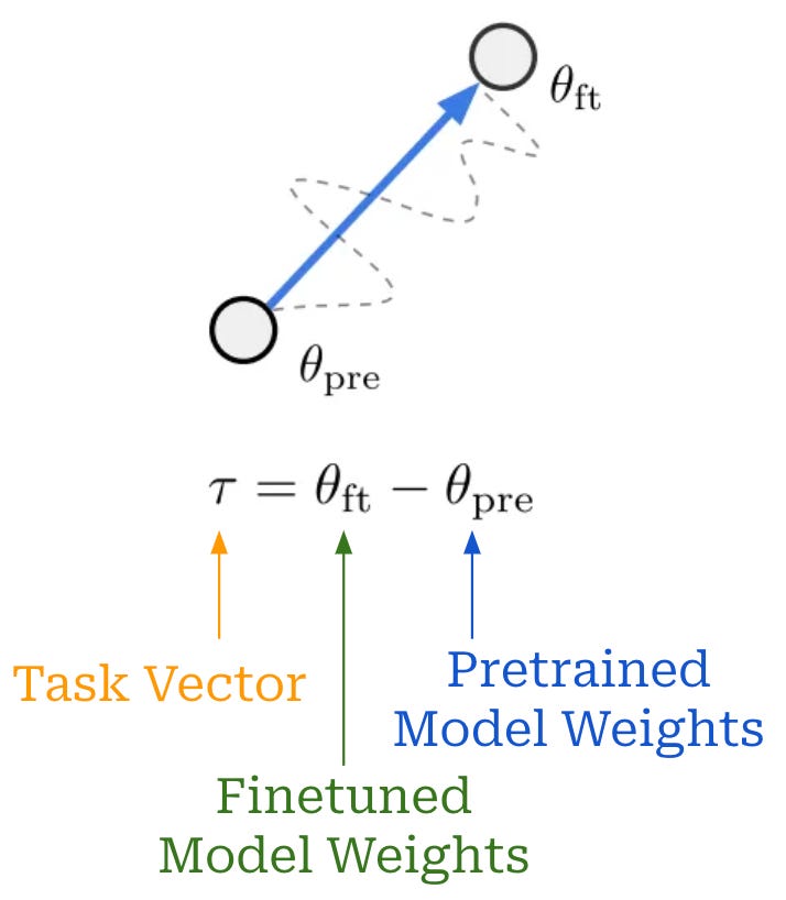
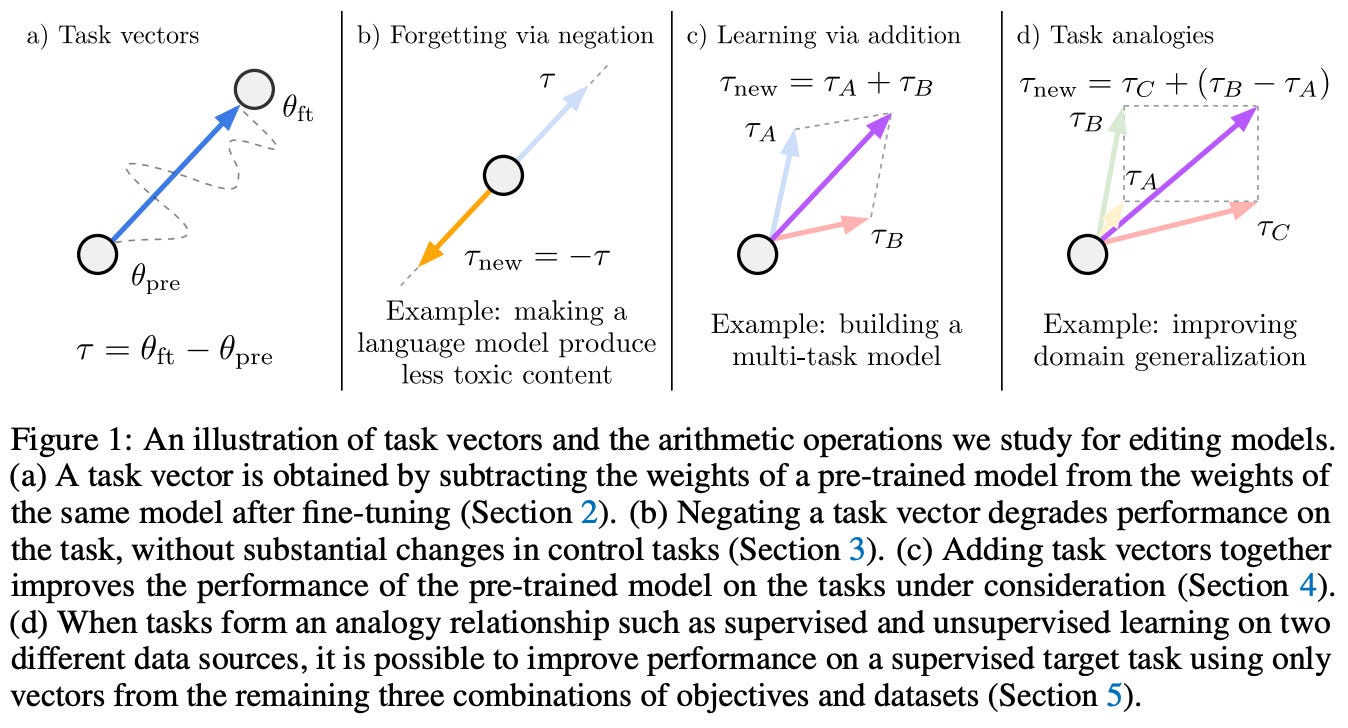
What is a task vector? The first concept introduced in [1] is a task vector, which simply refers to a vector that is obtained by subtracting a finetuned model’s weights from a pretrained model; see above. Intuitively, a task vector encodes all of the information needed to solve a task that is learned via finetuning. These task vectors live within the parameter space of a neural network, meaning that they are the same size and shape as the weights of the model we are trying to edit.
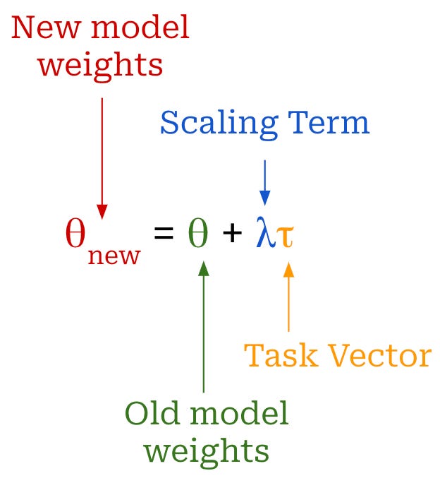
In [1], we see that these task vectors can be used to change the behavior of a pretrained model—task vectors are a simple and cheap alternative to prompting or finetuning. In particular, we can edit a model by performing arithmetic between the model’s parameters and a task vector, as shown above. The scaling term is typically tuned via a hold-out validation set. Intuitively, these task vectors move the parameters of our model towards those of a model with the desired behavior. This approach requires that all models share the exact same architecture.
Types of arithmetic. Beyond basic addition, we see in [1] that there are several forms of meaningful arithmetic that can be performed with task vectors; see above. We can add a task vector to learn a new skill or negate a task vector to eliminate a skill. We can even add or negate several task vectors at once!
“Negating a vector can be used to remove undesirable behaviors or unlearn tasks, while adding task vectors leads to better multi-task models, or even improves performance on a single task.” - from [1]
Going further, authors find in [1] that analogies between task vectors hold as well. Assume we have four tasks A, B, C, and D with a analogous relationship given by “A is to B as C is to D”. Then, we can improve performance on task D using the task vector shown below. Here, we construct a task vector by:
Finding the difference in task vectors between tasks A and B.
Adding this difference to the task vector for task C.
Experimental results. Task vectors are applied to numerous types of models in [1], including both LLMs and specialized models (e.g., image and text classifiers). We see that adding and negating task vectors is clearly effective. For example, we can obtain a toxicity task vector by finetuning an LLM on toxic text. Then, we can make an LLM less toxic by negating this task vector; see below.
We can also forget certain image classification tasks via negation, as well as learn new tasks—even multiple tasks at the same time—via addition. For example, the image below show how pairs of task vectors can improve an image classifier’s performance on downstream tasks, while the table shows that tasks vectors obtained from an LLM that has been finetuned on a downstream task can be used to improve a model’s performance on that task without extra finetuning!
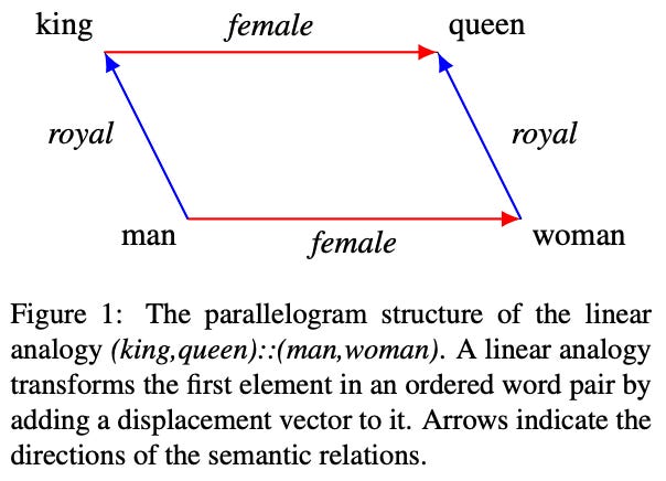
Additionally, these improvements in performance seem to avoid associated degradations in performance on control tasks—the model does not get worse in other areas as a result of the task vector. Similar experimental results are observed for analogous task vectors, where we see that most task vectors are orthogonal and can be used to generalize to new domains. In many ways, this analysis is reminiscent of early analysis of word vectors, where we observed similar analogous relationships between the vectors of associated words; see below.
Key benefits. Compared to prompting or finetuning, editing models via task arithmetic is cheap and easy. We do not need any external data or GPUs for training. Rather, we just need access to a finetuned model—many of which are already available online! Task arithmetic only requires element-wise operations on the model’s weights to quickly experiment with different task vectors. So, we can easily re-use or transfer knowledge from models that are openly available.
TIES-Merging: Resolving Interference When Merging Models [2]
“When merging a parameter that is influential for one model but redundant (i.e. not influential) for other models, the influential value may be obscured by the redundant values, lowering the overall model performance.” - from [2]
Given the proliferation of task-specific, finetuned models online, model merging is a promising technique that could help to consolidate these models. However, the performance of basic model merging techniques (e.g., averaging or weighted averaging of parameters) tends to degrade as we merge larger numbers of models. In [2], authors study the task vector-based model merging regime [1] and identify that performance degradations due to model merging are largely caused by “interference” that occurs between model parameters during the merging process. In particular, two key sources of interference are identified:
Redundant parameters: many parameters in a task vector are redundant, and removing these parameters does not impact performance.
Sign disagreements: certain parameters may have a positive value for some models and negative value for others, which causes a conflict.
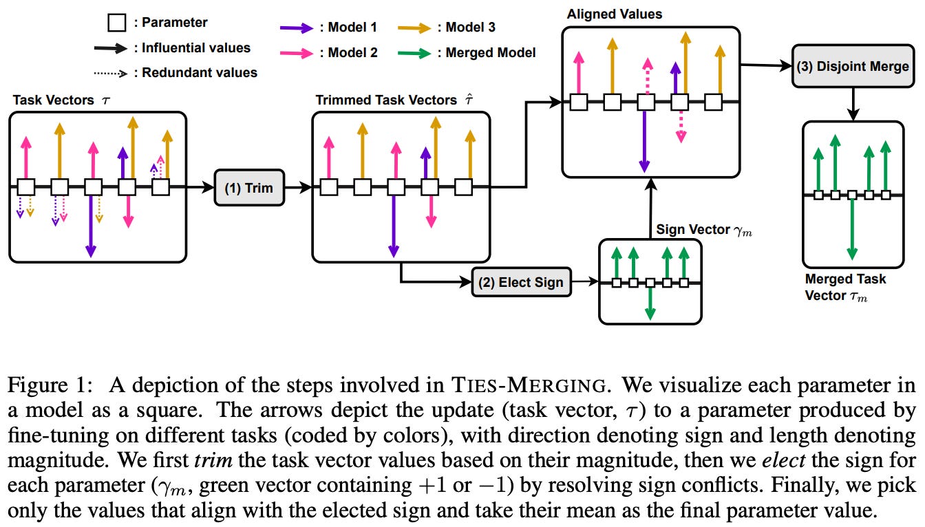
A schematic depiction of these different interference patterns is provided below.
To prove that this interference is occurring, we can just study basic properties of model parameters. In the (left) figure below, we first see that model performance is largely determined by a small group of (high magnitude) parameters, while most other parameters are redundant—meaning that they do not impact the model’s performance when removed12. Similarly, we see that sign conflicts are very common and become more common as the number of models considered is increased.
Dealing with interference. The method devised in [2] for mitigating interference, called TrIm, Elect Sign, and Merge (TIES-Merging), adds three additional steps to the task vector-based model merging process:
Trim: retain only influential weights (i.e., the top
K% of highest-magnitude values) in each task vector and set others to zero.Elect Sign: choose the sign of total highest magnitude for each element across task vectors—resulting in a sign vector13—by taking a element-wise sum across task vectors and seeing whether each resulting element is positive or negative.
Disjoint Merge: take the average of task vector values that agree with the majority sign, thus ignoring parameters that are either trimmed or have a sign conflict.
Once we have completed these three additional steps, we can perform model merging normally with the resulting task vector. The three steps within TIES-Merging are depicted below. Interestingly, we see in [2] that maintaining only the top 20% of task vector components yields stable performance—indicating that a large majority of task vector components are redundant!
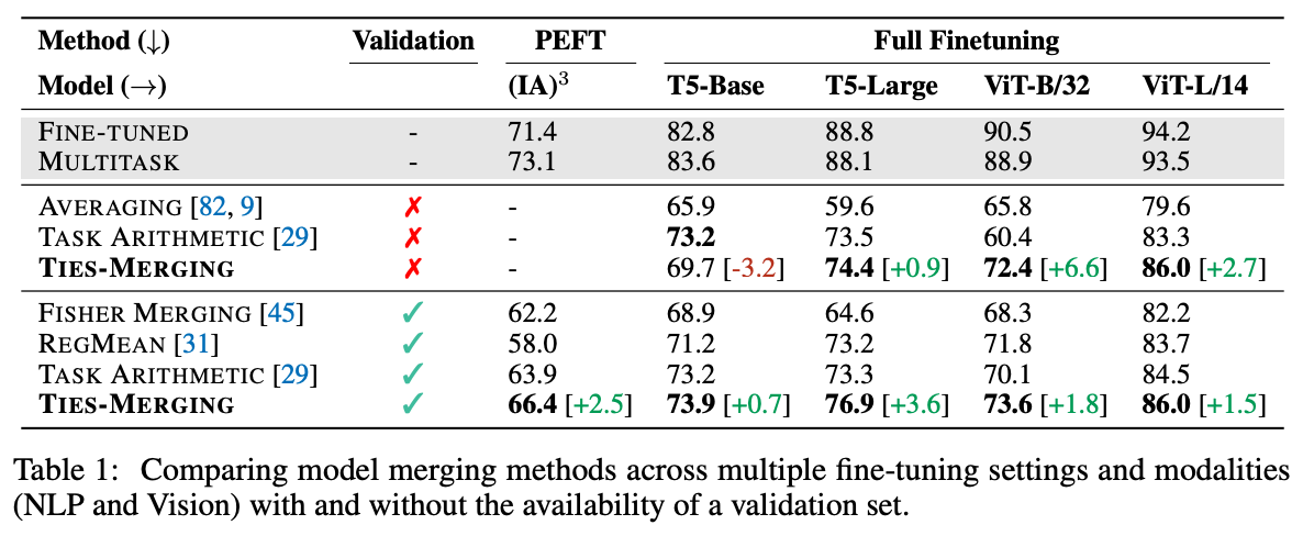
Less interference is beneficial. When TIES-merging is analyzed empirically, there are a variety of interesting findings from which we can learn. Overall, we see that TIES merging yields a clear benefit across a variety of experimental seeings; see below. In particular, TIES works well for multiple modalities (text and vision) and is even compatible with parameter-efficient finetuning.
Compared to baseline techniques, TIES-merging is also found to generalize better to new tasks and have improved scaling properties as the number of models being merged is (reasonably) increased; see below.
Both components of TIES-Merging—removing redundant parameter and electing a majority sign—are important, but properly estimating the majority sign seems to be especially important; e.g., flipping the sign of high magnitude parameters drastically deteriorates performance. Additionally, authors include interesting experiments in [2] that craft an oracle for estimating the majority sign by taking the sign of a model trained in a multi-task fashion. Using this sign oracle during the election process of TIES-Merging is actually found to improve performance!
Further finetuning. To go beyond the traditional model merging setup, we can perform extra finetuning with a model that is obtained via merging. In this domain, TIES-merging is shown in [2] to provide us with a better starting point. In particular, models obtained via TIES-Merging outperform those obtained via baseline merging techniques after further finetuning; see below.
Language Models are Super Mario: Absorbing Abilities from Homologous Models as a Free Lunch [3]
“In XMen’s Apocalypse, the character can absorb the powers of other mutants to strengthen himself… the protagonist in Super Mario can gain superpowers by absorbing in-game items… we astonishingly find that language models (LMs) can enhance their capabilities by absorbing other models without retraining or even GPUs.” - from [3]
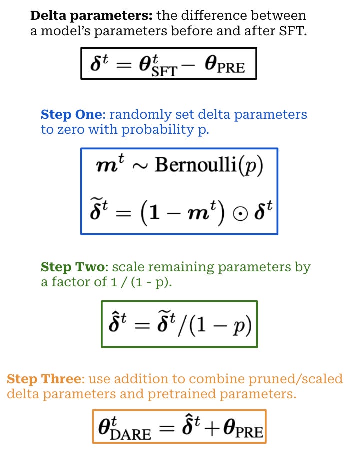
Authors in [3] propose an addition to existing model merging methods that is especially effective for language models that have underwent supervised finetuning (SFT). When studying the different in parameters values between the base model and the model obtained after SFT—referred to as “delta parameters”—we see (again) in [3] that these parameter values have a lot of redundancy. As a result, many of these delta parameters can be eliminated via a technique proposed in [3], called Drop And REscale (DARE). The DARE process makes language models finetuned with SFT much more amenable to model merging.
What is DARE? The concept proposed in [3] is actually very simple. We just:
Randomly drop delta parameters (with probability
p).Rescale remaining parameters by a factor of
1 / (1 - p).Add the remaining pruned and scaled parameters to the weights of the pretrained base model.
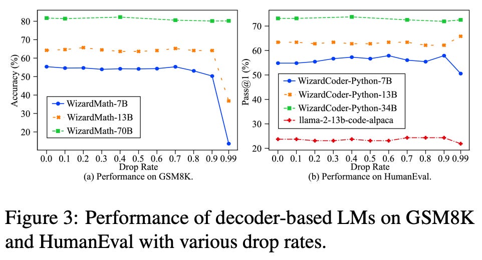
These steps are outlined in the figure above. Notably, DARE is not a model merging technique. Rather, it is a technique for sparsifying delta parameters within an SFT model that is found empirically to have minimal impact on the resulting model’s performance. In fact, we can even use DARE to eliminate up to 99% of delta parameters for sufficiently large language models; see below. Such a finding demonstrates that delta parameters for SFT models are highly redundant.
Application to model merging. Although DARE itself is not a model merging technique, it is a useful plug-in for existing methods (e.g., TIES-Merging [2]). The delta parameters considered by DARE are identical to the task vectors considered by prior model merging techniques [1]. DARE sparsifies these task vectors without damaging the underlying model’s performance, which mitigates interference when the parameters of these models are actually merged! Assuming models being merged share the same backbone, the chance of interference is much lower when merging multiple models to which DARE has been applied—many of the delta parameters within these models will have been set to zero.
In [3], authors merge various flavors of language models—including both encoder-only and decoder-only models—with and without DARE. In the table above, we see that using DARE on top of existing model merging techniques for decoder-only LLMs tends to (slightly) improve the performance of the merged model. This difference in performance is more noticeable when merging several specialized models (e.g., instruction-following, math, and code models).
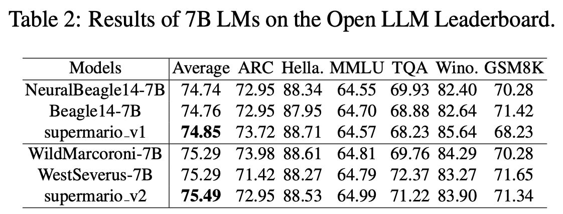
To demonstrate its utility, DARE is used to create two 7B parameter LLMs by merging the NeuralBeagle / Turdus (supermario-v1) and WildMorcoroni / WestSeverus (supermario-v2) models. These models achieve top performance (at the time) among 7B models on the Open LLM leaderboard; see below.
The performance impact of DARE is even more noticeable for encoder-only models; see below (left). The performance of several specialized models can be maintained after merging even while keeping only a small number of delta parameters from each SFT model. However, the rescaling step of DARE is essential to performance under higher levels of sparsity; see below (right).
Can we always use DARE? DARE is a sparsification technique that provides useful insight about language models (i.e., delta parameters are very sparse) and can be used to yield a slight boost in model merging performance. However, DARE is not applicable to models in every setting. We see in [3] that language models finetuned via SFT have uniquely small delta parameters—minimal modifications are made to the pretrained LLM. When similar models are finetuned using a continued pretraining setup, we observe delta parameters with much larger magnitudes. As a result, applying DARE in this setting is more damaging to performance, especially when dropping larger ratios of delta parameters.
“This finding further confirms that SFT primarily unlocks the abilities of pre-trained LMs, rather than introducing new capabilities.” - from [3]
This finding has connections to prior analysis of the Superficial Alignment Hypothesis [4], which posits that:
All of a language model’s knowledge is learned during pretraining.
Alignment serves the purposes of teaching the model how to properly surface this knowledge (e.g., style, format, tone, etc.).
Alignment can be highly data-efficient because of this.
With this in mind, we should not be too surprised that language models finetuned with SFT—an alignment technique—show a relatively small delta compared to the pretrained model. Similarly, continued pretraining should have a larger delta, as it usually serves the purpose of injecting new knowledge into the model.
WARP: On the Benefits of Weight Averaged Rewarded Policies [10]
“While weight averaging was initially mostly used for discriminative tasks… it is now becoming popular for generative tasks; its use in KL-constrained RLHF has already shown preliminary successes.” - from [10]
As we have seen, model merging has a long history of interesting applications and techniques within deep learning. Recently, however, we have begun to see model merging explored in the context of LLM alignment. The success of model merging in this domain has had a noticeable impact on pipelines used for training frontier models—merging is becoming a commonly-used component.
Refresher on alignment. Most LLMs are trained using a three-stage process that includes pretraining, supervised finetuning (SFT) and reinforcement learning from human feedback (RLHF); see below. During pretraining, we train the language model—using next token prediction—over large amounts of unlabeled text to build a large base of knowledge within the model. From here, we perform SFT and/or RLHF. These algorithms power the LLM finetuning (or alignment) process and are less computationally expensive relative to pretraining.
Typically, we first perform SFT over a (relatively) small14, high-quality set of examples, providing us with a better “starting point” for RLHF. Then, we apply RLHF in an iterative fashion by continually collecting new batches of preference data and further finetuning the model. The purpose of alignment is not to instill new knowledge within the LLM, but rather to teach the model how to surface its existing knowledge to human users in a preferable manner.
Why do we need model merging? When using RLHF, we usually add a Kullback-Leibler (KL) divergence term (shown above) to the objective being used, which measures the distance between the current model and the SFT model—or some other anchor model. At a high level, this divergence term captures how much the model has changed during training with RLHF. By making sure this term does not become too large, we can avoid issues like:
Forgetting of knowledge from pretraining (i.e., the alignment tax [28]).
Reward hacking (e.g., verbose, unsafe, or flawed outputs).
Decline in the diversity of model outputs [29].
However, adding this divergence term also hinders the reward optimization, forming a tradeoff between the model’s final reward and the KL divergence. As outlined in [10], model merging is an effective technique for finding better tradeoffs between the KL divergence and reward during finetuning with RLHF!
Weight Averaged Rewarded Policies (WARP) [10], depicted in the figure above, incorporates three types of model merging at three different phases of the LLM alignment process:
We use an Exponential Moving Average (EMA) of model weights as an anchor for the KL divergence during finetuning with RLHF.
We independently finetune
Mmodels via RLHF, then merge the policies using task vectors and spherical linear interpolation (SLERP); see here and above.We linearly interpolate the result towards the (SFT) initialization.
SLERP [37] can also be plugged in to any of the other model merging techniques we have seen so far as an alternative to linear interpolation.
“Merging task vectors, either with SLERP or LERP, combines their abilities. The difference is that SLERP preserves their norms, reaching higher rewards than the base models.” - from [10]
This multi-stage merging approach—see below for a full outline of each stage—uses several of the model merging techniques we’ve seen so far, including EMA [24, 27], weight averaging [22], task vectors [1], and WiSE-FT [8].
WARP has additional training costs—due to the need to independently train several models via RLHF—but has no additional memory or compute requirements at inference time. Model merging yields a unique benefit at each stage of the WARP algorithm. Using the EMA of model weights as an anchor for KL divergence allows the divergence constraint to be relaxed over time—weights are tied to the SFT model early on and gradient updates become more aggressive at the end of training.
Similarly, using SLERP to merge the weights of several RLHF models yields an improvement in reward, while interpolating back towards the SFT initialization finds a better tradeoff between reward and KL divergence. WARP is applied in an iterative fashion by performing several “rounds” of finetuning, where the final model at each iteration is used as an initialization for the next. This iterative approach matches the usual strategy used for RLHF within the literature.
Using WARP in practice. The result of this combination of merging techniques is a model that achieves the best possible tradeoff between KL and reward. The benefits of WARP are empirically validated in [10] using Gemma [30]. Models are evaluated in terms of i) their final reward and ii) KL divergence with respect to the SFT initialization. From experiments, we see that WARP achieves a better reward-KL tradeoff compared to other RL-based alignment techniques; see above. Due to this finding, WARP was officially adopted within the alignment process used for the more recent Gemma-2 model [31]; see here for more details.
“We periodically reset the online model to an exponentially moving average (EMA) of itself, then reset the EMA model to the initial model.” - from [47]
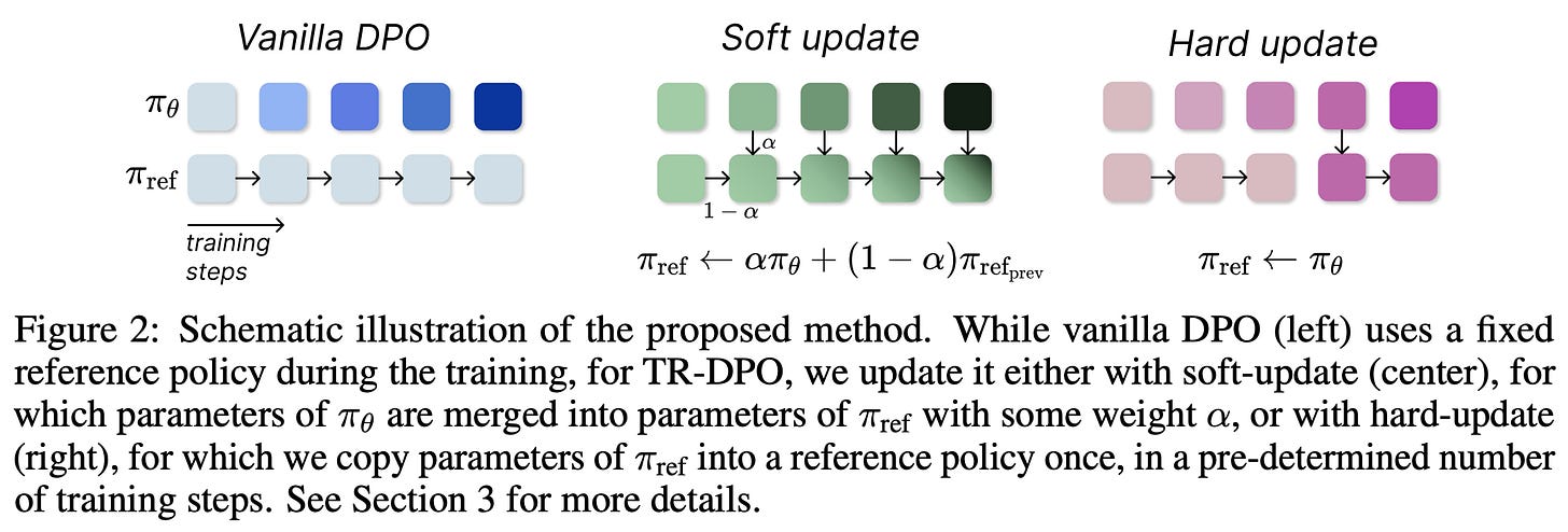
What came before this? Authors in [10] were not the first to try to address this balance between reward and KL. Elastic reset [47] eliminates KL divergence from the RLHF objective and instead periodically resets the model weights to the EMA of itself throughout the finetuning process, which enables higher rewards to be achieved with less drift. Alternatively, authors in [48] propose a similar strategy for updating the anchor model within RLHF by periodically setting the anchor model equal to the EMA of model weights; see above. Notably, this update strategy is quite similar to the first stage WARP.
In [50], we see that merging pre and post-RLHF models—similarly to WiSE-FT or stage three of WARP—is an effective method of mitigating the alignment tax, allowing us to achieve high reward without significantly degrading benchmark performance relative to the pre-RLHF model. Authors also perform some analysis to show that the benefits of model averaging are related to an increase in feature diversity, which aligns with findings in [42]. Going further, we see in [51] that LLMs finetuned via SFT also tend to suffer from an alignment tax, which can be solved via a model merging strategy that:
Trains many SFT “sub-models” on different subsets of instruction-following data, thus mitigating sources of bias in the dataset used for SFT.
Merges all SFT sub-models into a single model via a weighted average.
As we can see from this work, the ideas explored in WARP have their foundations in prior research. However, WARP combines these ideas into a novel, unified framework that is highly effective in the LLM alignment domain.
Advanced Topics in Model Merging Research
Beyond the core papers explored above, a variety of research has been published on the topic of model merging in the last few years, especially due to the technique’s popularity in the LLM domain. In this section, we outline several recent areas of research related to model merging that are especially interesting.
Merging reward models. So far, we have seen several examples of techniques for integrating model merging into the preference tuning process for LLMs [10, 47, 48, 50]. A few recent papers have focused on the more specific application of merging for creating better reward models—a single step within the RLHF process. The two primary techniques in this space, which are quite similar to each other, are called Weight Averaged Reward Models (WARM) [52] and Reward Soups [53]. This research, which aims to lessen the chances of reward hacking, independently trains several reward models with different hyperparameters and merges all of these models together; see above. Reward models obtained via such a merging strategy are found to be more robust and reliable compared to individual reward models, leading to improved downstream results with RLHF.
Merging independent models. Usually, we merge models that are derived from the same pretrained model. These models share the same architecture and are guaranteed to be linearly mode connected. However, recent work has explored merging models that are trained independently. The foundation of this work is the idea of permutation invariance [38, 39], which claims that all models trained to convergence via SGD—even those that are independently trained—lie in the same region of the loss landscape if we permute (or shuffle) their weights properly; see above. If we find the proper permutation such that this is the case (i.e., see [38] for an algorithm to do this), these models are linearly mode connected—as shown in [39]—and we can successfully merge their weights.
More recent work [40] has also explored distillation-based strategies for merging several LLMs with different architectures by i) computing the outputs of several source LLMs for each input text and ii) training a target LLM to align with the output distributions produced by each of the source models; see above.
Evolutionary model merging. Evolutionary algorithms are a class of optimization techniques that serve as an alternative to gradient-based optimization. Instead of using gradient descent to train a model, we simply evolve a population of models by iteratively selecting (and modifying) a dynamic, high-performing—as measured by a loss or objective function—subset of models within the population; see here for an overview of this topic. In [32], authors explore the intersection of evolutionary algorithms and model merging, finding that we can use these techniques to automatically discover effective combinations of open-source models; see above. In particular, we can evolve the weights used to merge a group of models at each layer, finding a more optimal model combination during the merging process.
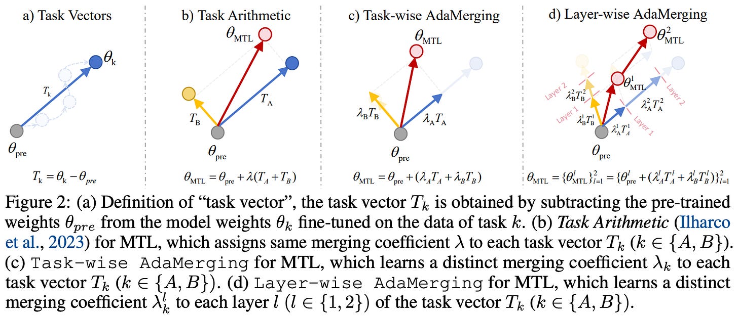
Adaptive (or automatic) merging. Instead of evolving the coefficients used for model merging, authors in [34] show that we can use unsupervised methods to discover optimal merging parameters without the need for any training data. This technique, called AdaMerge, is based on the idea of entropy minimization. We take a bunch of unlabeled data, compute the model’s predictions on this data, and train the merging coefficients to minimize the entropy of these predictions; see above. Given that this technique is mostly applied to classification tasks with ViT models in [34], this means that we train the model to place most of its probability mass on a single class, as opposed to being “unsure” (i.e., assigning relatively high probability to several classes). This technique is shown to yield competitive results in the multi-task learning domain for classification models.
Passthrough merging. LLM practitioners have recently explored the idea of combining several LLMs into one by simply concatenating their layers. This approach yields models with weird parameter counts (e.g., Goliath-120B or Solar-10.7B), referred to as Frankenstein models (or “FrankenMerges”) by the AI community; see here for details. Passthrough merging has not been explored extensively in the literature, but authors in [33] do discuss this technique—referred to as depth up-scaling in their report—for Solar-10.7B; see above. Nonetheless, passthrough merging has been used extensively by practitioners, resulting in the creation of several impressive models when paired with additional training.
Concluding Thoughts
We have seen a lot of information within this overview, but the fundamental idea we have covered is incredibly simple—taking a (weighted) average of weights for a group of models is an effective way of combining them. This simple idea has spawned an entire field of research, impacting a variety of important topics like neural network training and optimization, transfer learning, sparsity and pruning, LLM alignment, and more. To summarize some of this amazing research, a few basic takeaways from model merging research over the years have been outlined below.
A new technique? The idea of model merging is not new whatsoever. In fact, this idea is nearly as old as the concept of an ensemble [7]. The intuition behind model merging is quite simple. We know that forming an output-space ensemble of several machine learning models can benefit performance, but this approach increases inference costs. Instead, we can take a weight-space ensemble via a (weighted) average of the models’ parameters, forming a single merged model with performance that rivals that of an ensemble. Many papers have extended this concept over time, but the fundamental idea and intuition remains the same!
Why does this work? To understand the effectiveness of model merging, we need to understand two fundamental concepts: mode connectivity and sparsity. Linear mode connectivity tells us that different finetuned models lie in a similar basin of the loss landscape and that all models obtained via interpolation of these models have constant performance. For this reason, merging—or interpolating—models just yields another high-performing model! Plus, the fact that deep networks (including LLMs) exhibit high levels of sparsity implies that the likelihood of a conflict occurring between merged model parameters is relatively low.
Where should we start? The most basic implementation of model merging that we can derive is a uniform average of model weights, which works well in many cases. Beyond this simple approach, the fundamental idea behind model merging is best characterized by the concept of a task vector [1]. After creating task vectors for different finetuned models, we can perform arbitrary arithmetic and create a variety of interesting model combinations or merges, as well as perform (weighted) model averaging. To determine the optimal weights to use for model merging, we can simply measure performance on a hold-out validation set.
Advanced strategies. If simple model merging techniques based upon averaging or task vectors do not yield our desired result, we can explore more advanced model merging techniques, such as TIES, DARE, SLERP, and more. These strategies improve upon baseline performance by increasing sparsity, accounting for interference between merged parameters, maintaining useful geometric properties of merged model weights, and more. Going further, new merging techniques (e.g., Passthrough merging) are being proposed all the time. We should always try simple techniques first, but more advanced merging strategies have been applied successfully in practice and may be beneficial to some use cases.
New to the newsletter?
Hi! I’m Cameron R. Wolfe, Deep Learning Ph.D. and Machine Learning Scientist at Netflix. This is the Deep (Learning) Focus newsletter, where I help readers better understand important topics in AI research. If you like the newsletter, please subscribe, share it, or follow me on X and LinkedIn!
Bibliography
[1] Ilharco, Gabriel, et al. "Editing models with task arithmetic." arXiv preprint arXiv:2212.04089 (2022).
[2] Yadav, Prateek, et al. "Ties-merging: Resolving interference when merging models." Advances in Neural Information Processing Systems 36 (2024).
[3] Yu, Le, et al. "Language models are super mario: Absorbing abilities from homologous models as a free lunch." Forty-first International Conference on Machine Learning. 2024.
[4] Zhou, Chunting, et al. "Lima: Less is more for alignment." Advances in Neural Information Processing Systems 36 (2024).
[5] Wortsman, Mitchell, et al. "Model soups: averaging weights of multiple fine-tuned models improves accuracy without increasing inference time." International conference on machine learning. PMLR, 2022.
[6] Dietterich, Thomas G. "Ensemble methods in machine learning." International workshop on multiple classifier systems. Berlin, Heidelberg: Springer Berlin Heidelberg, 2000.
[7] Utans, Joachim. "Weight averaging for neural networks and local resampling schemes." Proc. AAAI-96 Workshop on Integrating Multiple Learned Models. AAAI Press. Citeseer, 1996.
[8] Wortsman, Mitchell, et al. "Robust fine-tuning of zero-shot models." Proceedings of the IEEE/CVF conference on computer vision and pattern recognition. 2022.
[9] Jang, Dong-Hwan, Sangdoo Yun, and Dongyoon Han. "Model Stock: All we need is just a few fine-tuned models." arXiv preprint arXiv:2403.19522 (2024).
[10] Ramé, Alexandre, et al. "WARP: On the Benefits of Weight Averaged Rewarded Policies." arXiv preprint arXiv:2406.16768 (2024).
[11] Garipov, Timur, et al. "Loss surfaces, mode connectivity, and fast ensembling of dnns." Advances in neural information processing systems 31 (2018).
[12] Frankle, Jonathan, et al. "Linear mode connectivity and the lottery ticket hypothesis." International Conference on Machine Learning. PMLR, 2020.
[13] Neyshabur, Behnam, Hanie Sedghi, and Chiyuan Zhang. "What is being transferred in transfer learning?." Advances in neural information processing systems 33 (2020): 512-523.
[14] Rofin, Mark, Nikita Balagansky, and Daniil Gavrilov. "Linear interpolation in parameter space is good enough for fine-tuned language models." arXiv preprint arXiv:2211.12092 (2022).
[15] Sun, Mingjie, et al. "Massive activations in large language models." arXiv preprint arXiv:2402.17762 (2024).
[16] Frankle, Jonathan, and Michael Carbin. "The lottery ticket hypothesis: Finding sparse, trainable neural networks." arXiv preprint arXiv:1803.03635 (2018).
[17] LeCun, Yann, John Denker, and Sara Solla. "Optimal brain damage." Advances in neural information processing systems 2 (1989).
[18] Hassibi, Babak, David G. Stork, and Gregory J. Wolff. "Optimal brain surgeon and general network pruning." IEEE international conference on neural networks. IEEE, 1993.
[19] Frantar, Elias, and Dan Alistarh. "Sparsegpt: Massive language models can be accurately pruned in one-shot." International Conference on Machine Learning. PMLR, 2023.
[20] Sun, Mingjie, et al. "A simple and effective pruning approach for large language models." arXiv preprint arXiv:2306.11695 (2023).
[21] Tim Dettmers, Mike Lewis, Younes Belkada, and Luke Zettlemoyer. LLM.int8(): 8-bit matrix multiplication for transformers at scale. In NeurIPS, 2022.
[22] Izmailov, Pavel, et al. "Averaging weights leads to wider optima and better generalization." arXiv preprint arXiv:1803.05407 (2018).
[23] David Ruppert. Efficient estimations from a slowly convergent robbins-monro process. Technical report, Cornell University Operations Research and Industrial Engineering, 1988.
[24] Diederik P Kingma and Jimmy Ba. Adam: A method for stochastic optimization. arXiv preprint arXiv:1412.6980, 2014.
[25] Laine, Samuli and Aila, Timo. Temporal Ensembling for Semi-Supervised Learning. arXiv:1610.02242 [cs], October 2016. arXiv: 1610.02242.
[26] Tarvainen, Antti, and Harri Valpola. "Mean teachers are better role models: Weight-averaged consistency targets improve semi-supervised deep learning results." Advances in neural information processing systems 30 (2017).
[27] Sanyal, Sunny, et al. "Early weight averaging meets high learning rates for llm pre-training." arXiv preprint arXiv:2306.03241 (2023).
[28] Ouyang, Long, et al. "Training language models to follow instructions with human feedback." Advances in neural information processing systems 35 (2022): 27730-27744.
[29] Kirk, Robert, et al. "Understanding the effects of rlhf on llm generalisation and diversity." arXiv preprint arXiv:2310.06452 (2023).
[30] Team, Gemma, et al. "Gemma: Open models based on gemini research and technology." arXiv preprint arXiv:2403.08295 (2024).
[31] Team, Gemma, et al. "Gemma 2: Improving open language models at a practical size." arXiv preprint arXiv:2408.00118 (2024).
[32] Akiba, Takuya, et al. "Evolutionary optimization of model merging recipes." arXiv preprint arXiv:2403.13187 (2024).
[33] Kim, Dahyun, et al. "Solar 10.7 b: Scaling large language models with simple yet effective depth up-scaling." arXiv preprint arXiv:2312.15166 (2023).
[34] Yang, Enneng, et al. "Adamerging: Adaptive model merging for multi-task learning." arXiv preprint arXiv:2310.02575 (2023).
[35] Rame, Alexandre, et al. "Diverse weight averaging for out-of-distribution generalization." Advances in Neural Information Processing Systems 35 (2022): 10821-10836.
[36] Ramé, Alexandre, et al. "Model ratatouille: Recycling diverse models for out-of-distribution generalization." International Conference on Machine Learning. PMLR, 2023.
[37] Ken Shoemake. Animating rotation with quaternion curves. In SIGGRAPH, 1985.
[38] Ainsworth, Samuel K., Jonathan Hayase, and Siddhartha Srinivasa. "Git re-basin: Merging models modulo permutation symmetries." arXiv preprint arXiv:2209.04836 (2022).
[39] Entezari, Rahim, et al. "The role of permutation invariance in linear mode connectivity of neural networks." arXiv preprint arXiv:2110.06296 (2021).
[40] Wan, Fanqi, et al. "Knowledge fusion of large language models." arXiv preprint arXiv:2401.10491 (2024).
[41] Cha, Junbum, et al. "Swad: Domain generalization by seeking flat minima." Advances in Neural Information Processing Systems 34 (2021): 22405-22418.
[42] Lin, Yong, et al. "Spurious feature diversification improves out-of-distribution generalization." arXiv preprint arXiv:2309.17230 (2023).
[43] Zaman, Kerem, Leshem Choshen, and Shashank Srivastava. "Fuse to forget: Bias reduction and selective memorization through model fusion." arXiv preprint arXiv:2311.07682 (2023).
[44] Eeckt, Steven Vander. "Weight averaging: A simple yet effective method to overcome catastrophic forgetting in automatic speech recognition." arXiv preprint arXiv:2210.15282 (2022).
[45] Lawson, Daniel, and Ahmed H. Qureshi. "Merging decision transformers: Weight averaging for forming multi-task policies." 2024 IEEE International Conference on Robotics and Automation (ICRA). IEEE, 2024.
[46] Nikishin, Evgenii, et al. "Improving stability in deep reinforcement learning with weight averaging." Uncertainty in artificial intelligence workshop on uncertainty in Deep learning. 2018.
[47] Noukhovitch, Michael, et al. "Language model alignment with elastic reset." Advances in Neural Information Processing Systems 36 (2024).
[48] Gorbatovski, Alexey, et al. "Learn your reference model for real good alignment." arXiv preprint arXiv:2404.09656 (2024).
[49] Xiao, Shitao, et al. "Lm-cocktail: Resilient tuning of language models via model merging." arXiv preprint arXiv:2311.13534 (2023).
[50] Lin, Yong, et al. “Mitigating the alignment tax of rlhf.” arXiv preprint arXiv:2309.06256 (2024).
[51] Fu, Tingchen, et al. "Disperse-Then-Merge: Pushing the Limits of Instruction Tuning via Alignment Tax Reduction." arXiv preprint arXiv:2405.13432 (2024).
[52] Ramé, Alexandre, et al. "Warm: On the benefits of weight averaged reward models." arXiv preprint arXiv:2401.12187 (2024).
[53] Rame, Alexandre, et al. "Rewarded soups: towards pareto-optimal alignment by interpolating weights fine-tuned on diverse rewards." Advances in Neural Information Processing Systems 36 (2024).
[54] Goddard, Charles, et al. "Arcee's MergeKit: A Toolkit for Merging Large Language Models." arXiv preprint arXiv:2403.13257 (2024).
Multi-task learning is an alternative technique that avoids this issue with increased inference cost. However, multi-task learning is not a clean alternative to a model ensemble, as the situations in which these two techniques would be applied can be different (e.g., we can create an ensemble of models trained on only one task).
The “deep learning era” in this context is considered to be anything after AlexNet was proposed in 2012.
Here, we assume that the networks have identical size / architecture and are just trained independently with different random seeds (potentially with some differences in other hyperparameters or settings).
By this, we mean that any weights along this connected path between the weights of the original networks yield a model with training and test accuracy that match or improve upon that of the original models.
This overview was the first Deep (Learning) Focus newsletter that was ever released!
Performance is measured both on the normal ImageNet test set, as well as several other ImageNet-related test sets with various distribution shifts (e.g., ImageNet-V2, ImageNet-R, ImageNet-Sketch, and more).
Prior state-of-the-art was 90.88%, achieved by CoAtNet. Today, state-of-the-art performance on ImageNet is slightly higher (around 92%).
See this paper as a great example of this phenomenon. We can outperform GPT-4 on particular target domains via finetuning!
Also, changing the coefficient used during model merging is easy! No extra training is required, whereas tweaking hyperparameters requires the model to be retrained.
Notably, all comparisons are performed in a layer-wise fashion, meaning that we only compare the weights of different finetuned models within the same layer.
This idea is explored in [22] for deep learning, but this technique in general is not new and can be seen in much earlier work; e.g., see [23] for an example.
Again, this finding has a strong connection to research on model pruning, where we see very similar observations!
This sign vector is just a vector with the same size as a task vector, where each element is either -1 or 1. The sign vector indicates the majority sign of each parameter across task vectors, as dictated by the elect sign step.
In most cases, the size of SFT datasets are within the range of a few thousand to a few tens of thousands of examples, but we have seen SFT applied successfully with as few as 1K examples (i.e., the algorithm is very data efficient).


















How you continue to keep up this quality every single time is beyond me. I'm convinced that you're three different people pretending to be one
Another incredible and detailed article. This substack is probably the most detailed I have seen as it relates to LLMs and deep learning concepts.