Language Model Training and Inference: From Concept to Code
Learning and implementing next token prediction with a causal language model...
Despite all that has been accomplished with large language models (LLMs), the underlying concept that powers all of these models is simple—we just need to accurately predict the next token! Though some may (reasonably) argue that recent research on LLMs goes beyond this basic idea, next token prediction still underlies the pre-training, fine-tuning (depending on the variant), and inference process of all causal language models, making it a fundamental and important concept for any LLM practitioner to understand.
“It is perhaps surprising that underlying all this progress is still the original autoregressive mechanism for generating text, which makes token-level decisions one by one and in a left-to-right fashion.” - from [10]
Within this overview, we will take a deep and practical dive into the concept of next token prediction to understand how it is used by language models both during training and inference. First, we will learn these ideas at a conceptual level. Then, we will walk through an actual implementation (in PyTorch) of the language model pretraining and inference processes to make the idea of next token prediction more concrete.
Relevant Background Concepts
Prior to diving into the topic of this overview, there are a few fundamental ideas that we need to understand. Within this section, we will quickly overview these important concepts and provide links to further reading for each.
The transformer architecture. First, we need to have a working understanding of the transformer architecture [5], especially the decoder-only variant. Luckily, we have covered these ideas extensively in the past:
More fundamentally, we also need to understand the idea of self-attention and the role that it plays in the transformer architecture. More specifically, large causal language models—the kind that we will study in this overview—use a particular variant of self-attention called multi-headed causal self-attention.
Training neural nets with PyTorch. The code we will look at in this overview is written in PyTorch and heavily relies upon distributed training techniques, such as distributed data parallel (DDP) training. To understand the basics of PyTorch and distributed training, check out the following articles:
Neural Nets in PyTorch [link]
PyTorch Distributed Overview [link]
Distributed Data Parallel in PyTorch [link]
Beyond basic (and distributed) neural network training in PyTorch, we will also see automatic mixed precision (AMP) training being used, which selectively adjusts the precision—between full precision (float32) and half precision (float16 or bfloat16)—within the neural net during training to improve efficiency. Put simply, we perform a lot of matrix multiplications within the neural net, and training is a lot faster if we can run some of these multiplications in lower precision. See here for a more extensive (and practical) overview of AMP.
Deep learning basics. This overview also requires a baseline understanding of neural networks, including how they are trained and used. To gain this knowledge, I highly recommend the Practical Deep Learning for Coders course from fast.ai, which is updated frequently and remains (in my opinion) the best practical introduction to deep learning that anyone can get1.
Understanding Next Token Prediction
We will now learn about next token prediction (also known as the standard language modeling objective)—the workhorse behind all causal language models. Within this section, we will first cover a few fundamental concepts related to tokenization, then we will overview the pretraining and inference processes for language models, as well as their relation to the concept of next token prediction.
Tokens and Vocabularies
In trying to understand next token prediction, the first question we might have is: What is a token? Put simply, a token is just a word or sub-word within a sequence of text. Given a sequence of raw text as input, the first step we take in using a language model is to tokenize this raw text, or break it into a sequence of discrete tokens; see below for an example.
To perform this tokenization, we rely upon a tokenizer. The tokenizer is trained over an unlabeled textual corpus to learn a fixed-size, unique set of tokens that exist. This fixed-size set of tokens is referred to as our vocabulary, and the vocabulary contains all tokens that are known by the language model. Usually, we should try to make sure that the data used to train the tokenizer accurately reflects the kind of data our model will see during training and inference. Given that the vocabulary has a fixed size, this ensures that the tokens we see in the wild are present within the language model’s vocabulary more often than not.
Tokenization techniques. Numerous different tokenization techniques exist; see here for an overview. For details on training and using popular tokenizers for LLMs, see this article that details the byte pair encoding (BPE) tokenizer—the most commonly-used tokenizer for LLMs. Another tokenization technique that has become recently popular is byte-level BPE (BBPE), which relies upon bytes (instead of textual characters) as the basic unit of tokenization.
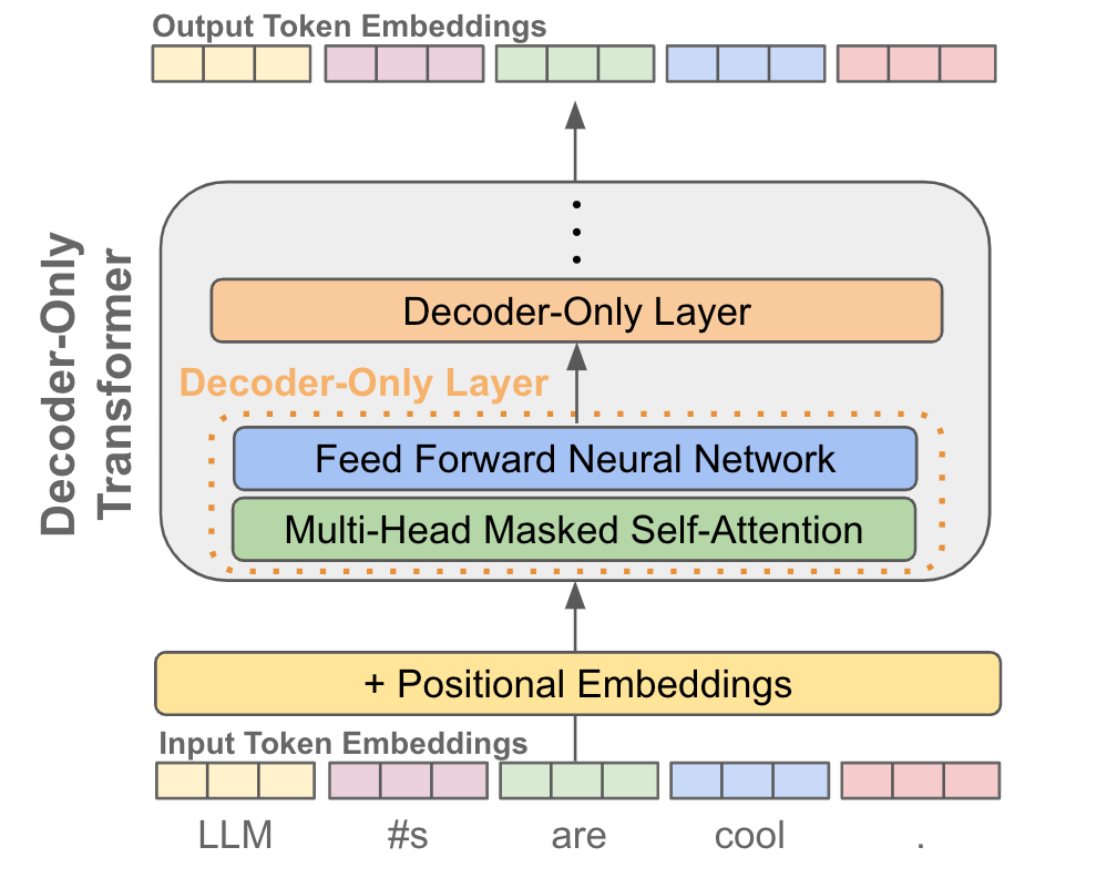
Token embeddings. Once we have tokenized our text, we look up the embedding for each token within an embedding layer that is stored as part of the language model’s parameters2. After this, the sequence of textual tokens constructed from our input becomes a sequence of token embedding vectors; see below.
There is one final step required to construct the input that is actually passed to our decoder-only transformer architecture—we need to add positional embeddings. Positional embeddings are the same size as token embeddings and treated similarly (i.e., they are stored as part of the language model and trained along with other model parameters). Instead of associating an embedding with each unique token, however, we associate an embedding with each unique position that can exist within a tokenized input; see below for a depiction.
We add these embeddings to the token embeddings at the corresponding position. Such additive positional embeddings are necessary because the self-attention operation does not have any way of representing the position of each token. By adding positional embeddings, we allow the self-attention layers within the transformer to use the position of each token as a relevant feature during the learning process. Recent research has explored novel techniques for injecting positional information into self-attention, resulting in techniques like RoPE [6].
Context window. Language models are pretrained with token sequences of a particular size, which is referred to as the size of the context window or the context length. This size—typically somewhere in the range of 1K to 8K tokens (though some models are much larger!)—is (usually) selected based hardware and memory constraints3. Given that we only learn positional embeddings for input of this length, the context window limits the amount of input data that an LLM can process. However, recent techniques like ALiBi [7] have been developed to enable extrapolation to inputs longer than those seen during training.
Language Model Pretraining
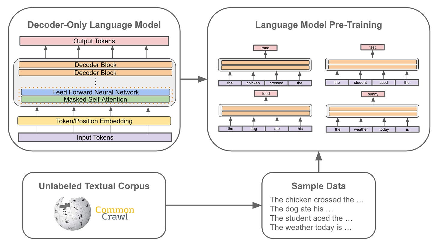
Language models are trained in several steps, as shown above. The first (and most computationally expensive) step is pretraining, which we will focus on within this overview. During pretraining, we get a large corpus of unlabeled text and train the model by i) sampling some text from the dataset and ii) training the model to predict the next word. This is a self-supervised objective due to the fact that no labels are required. Rather, the ground truth next token is already present within the corpus itself—the source of supervision is implicit. Such a training objective is referred to as next token prediction, or the standard language modeling objective.
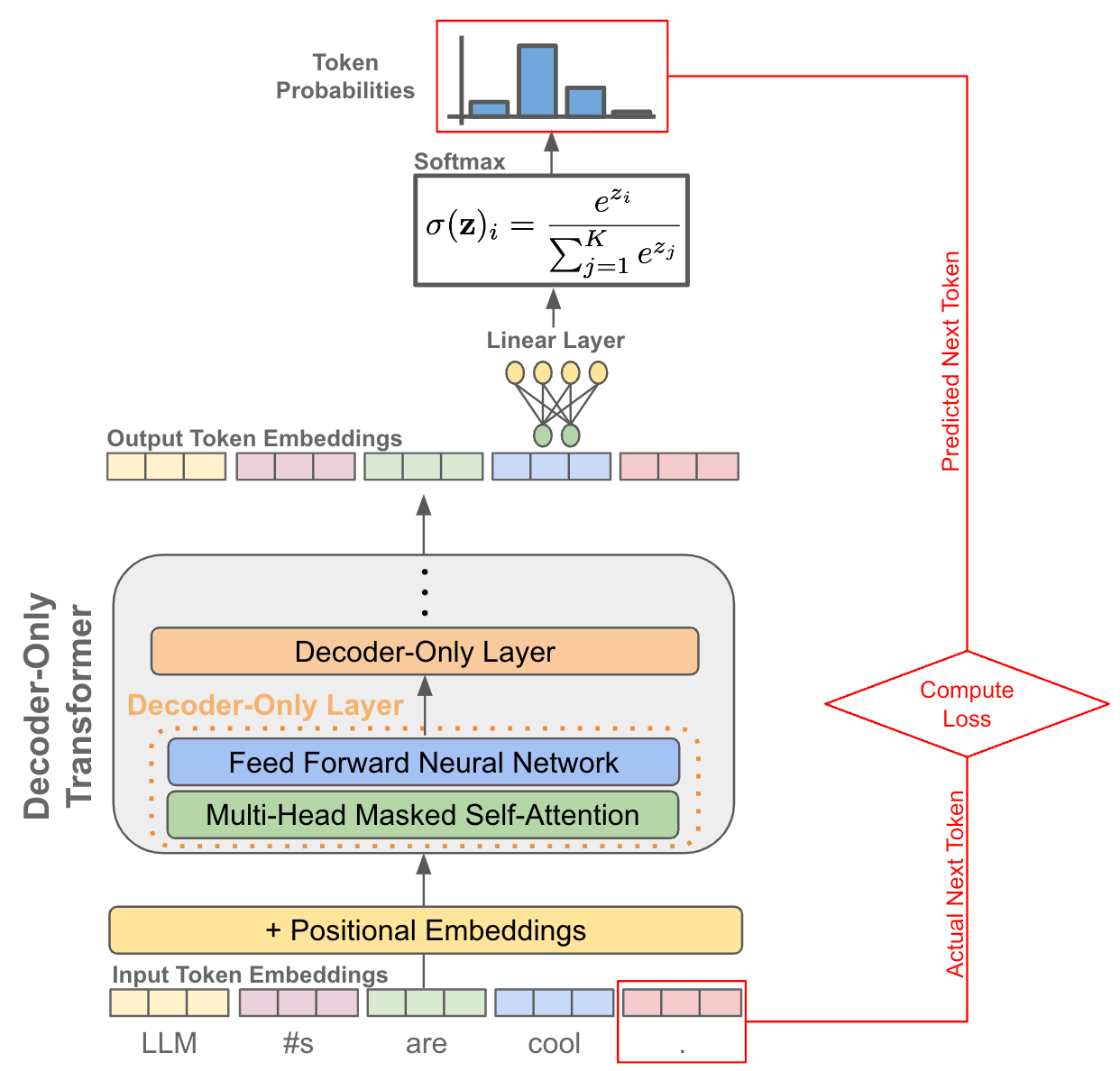
Predicting the next token. After we have our token embeddings (with position embeddings), we pass these vectors into a decoder-only transformer, which produces a corresponding output vector for each token embedding; see below.
Given an output vector for each token, we can perform next token prediction by i) taking the output vector for a token and ii) using this to predict the token that comes next in the sequence. See below for an illustration.
As we can see above, the next token is predicted by passing a token’s output vector as input to a linear layer, which outputs a vector with the same size as our vocabulary. After a softmax transformation is applied, a probability distribution over the token vocabulary is formed, and we can either i) sample the next token from this distribution during inference or ii) train the model to maximize the probability of the correct next token during pretraining.
Predicting tokens across a sequence. During pretraining, we don’t predict only a single next token. Rather, we perform next token prediction for every token in a sequence and aggregate the loss over them all. Due to the use of causal self-attention, each output token vector only considers the current token and those that come before it in the sequence. As such, next token prediction can be performed across an entire sequence using a single forward pass of the decoder-only transformer, as each token has no knowledge of tokens that come after it.
Autoregressive Inference Process
Now, we understand how to pretrain a language model, but next token prediction is also used when we are performing inference! Next token prediction underlies all aspects of training and using LLMs. Starting with an initial (possibly empty) input sequence or prefix, language models generate text by following an autoregressive next token prediction process (see above) with the following steps:
Predict the next token
Add the predicted token to the current input sequence
Repeat
Choosing next token. In the prior section, we’ve seen how a probability distribution over tokens is created. But, how do we actually choose the next token from this distribution? Typically, we just sample the next token from this distribution. However, numerous sampling strategies exist that add slight variations to this approach by modifying the probability distribution over tokens. The exact decoding approach varies depending upon the application, but the main concepts and strategies that we need to be familiar with are outlined below:
Creating a Minimal Implementation
Now that we understand the concept of next token prediction, we need to take the ideas we have learned and make them a bit more concrete. Within this section, we will examine an implementation—written in PyTorch—of pretraining and inference (using next token prediction) with an LLM. This implementation is derived from NanoGPT by Andrej Karpathy, which matches the specs of GPT-2 [1]. In addition to the implementation of NanoGPT provided on GitHub (linked above), there’s an awesome tutorial video to go with it; see below.
Although this model is small compared to most modern LLMs4, it serves as a great example of what language models look like in code. Here, we will study the implementation of NanoGPT and connect it to our discussion of next token prediction from previous sections.
The Decoder-Only Transformer
First, we will detail the implementation of our language model architecture, which is based upon a decoder-only transformer. First, we will overview the components of this architecture, moving from a single block of the model to the full, multi-layer architecture. Then, we will study how this model architecture can be used during pretraining and inference with next token prediction.
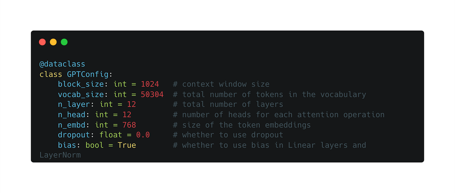
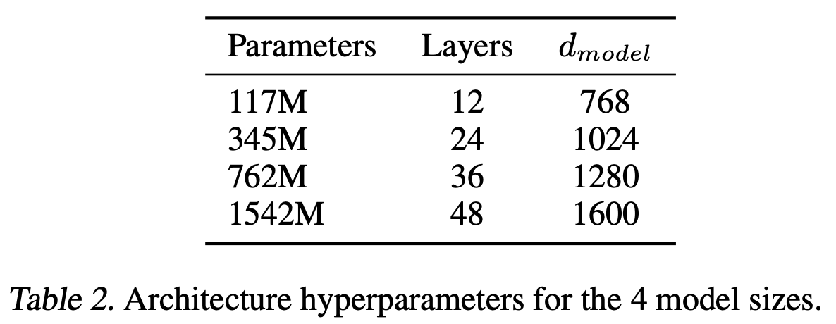
Model configuration. The first thing we need to look at is the configuration of our model architecture; see above. As we can see, the configuration is just a data class in Python that specifies the various hyperparameters of our architecture. The settings shown above correspond to those of the smallest model architecture explored within the GPT-2 paper [1], as shown in the table below.
This model contains only 117M parameters and is actually identical to the base transformer architecture used within the original GPT publication [2].
A single block. Next, we can look at the implementation of a single block within the decoder-only transformer architecture; see above. Here, we see that a decoder-only transformer block has two components:
For most language models (including NanoGPT), the feed-forward network is a two-layer model, where the hidden layer is slightly wider5 than the input layer. The block’s input is normalized prior to each of the two layers, and a residual connection is added between the layers. See below for an illustration.
Model definition. Now that we understand the structure of a decoder-only transformer block, we can look at NanoGPT’s full model definition. This definition is provided below, where we see the constructor for the model class.
As shown above, the LLM contains two different embedding layers—one to store token embeddings and one to store positional embeddings. There are 1024 positional embeddings, corresponding to the context length used to train NanoGPT (i.e., block_size setting in the configuration). The language model has 12 transformer blocks in total. The weights of the model are initialized normally, aside from a few special techniques adopted from GPT-2 [1].
Beyond the basic transformer architecture, there are extra dropout and LayerNorm modules that are used during the forward pass at the first/final layer of the LLM. Plus, we have a linear classification head that is used for next token prediction and shares weights with the token embedding layer. This weight sharing method, called weight tying [3], can improve performance while drastically decreasing the total number of parameters in the model6.
Implementing Next Token Prediction
Now that we understand the implementation of an LLM’s model architecture, we will take a look at a pretraining and inference implementation with the same architecture. Both pretraining (shown above) and inference rely upon a next token prediction strategy, and we will overview the implementation of next token prediction for each of these processes within this section.
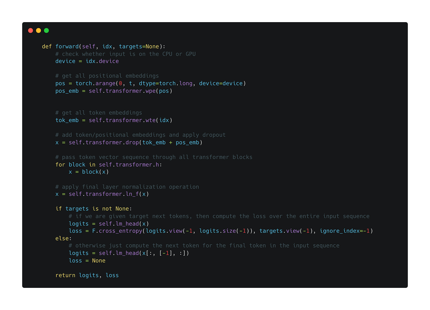
Forward pass. To understand how to train NanoGPT, we need to understand the model’s forward pass. There are two different types of forward passes that we can consider—one for training and one for inference. The code for NanoGPT’s forward pass (i.e., this method is part of the GPT model class provided previously) is shown below. First, we will consider how this forward pass is used during pretraining, then will return to the inference process later.
The forward pass operates as we might expect. We take two tensors as input:
Input tensor (
idx): a matrix where each row contains a sequence of token ids, representing a textual sequence to use for pretraining (or inference).Target tensor (
targets): similar to the input tensor, but each entry contains the ground truth next token id for each token in the input tensor.
Each of these tensors store an entire mini-batch that contains multiple sequences of text over which a training iteration is parallelized. Here, we will assume the target tensor is not None. This is always true during pretraining, while during inference we have no target and are just freely generating next tokens.
The first step in the forward pass it to construct a matrix corresponding to our positional and token embeddings; see above. The idx tensor contains token ids that can be directly used for lookup within the token embedding matrix. We have to manually construct index values to look up positional embeddings. Positional and token embeddings are added together, passed through a dropout layer, and passed through all transformer blocks. Then, a final LayerNorm operation is performed before computing the loss with the next token prediction objective.
The next token prediction process outputs a distribution over potential next tokens—using the linear lm_head module, where the transformer’s output vector for each token is used as input—for every token within the input sequence. Then, we apply a CrossEntropy loss to this result, thus training the model to correctly predict the next token at every position within the entire input sequence.
Performing inference. Beyond pretraining, we can can generate text with next token prediction. As explained previously, generating text with a language model is an autoregressive process that iteratively predicts each next token. To predict a token, NanoGPT follows the steps outlined below:
Perform a forward pass with the current input sequence
Scale the outputted logits according to the specified temperature
[Optional] Remove all but the
kmost likely tokens (i.e., Top-K sampling)Apply the softmax function
Sample the next token from the resulting distribution
Notably, the forward pass within the code above uses the same exact forward pass we defined previously, but no target tensor is specified within the input!
NanoGPT Training
Although distributed training is a complex topic that we will not be able to cover thoroughly in this overview, we will cover the practical highlights of NanoGPT’s pretraining process for the purpose of completeness. We typically distribute LLM training across multiple compute devices (e.g., GPUs or TPUs). At a high level, there are a few reasons that distributed training is desirable and/or necessary:
Pretraining is computationally expensive and we want to speed it up.
The size of the model might be too big to store on a single device.
The second case outlined above is especially applicable to the current generation of language models, which are quite large and typically cannot be stored on a single device. A variety of distributed training techniques exist that can handle these cases and speed up the training process; see here for a summary.
Distributed training setup. The full pretraining implementation is provided within the train.py file within NanoGPT’s repository. The model is trained using either using a single GPU or with a distributed data parallel (DDP) approach. The setup of this training framework is shown below.
As we can see, training with DDP requires that we simultaneously run multiple training processes7 that will communicate together. The number of processes is equal to the total number of GPUs that we have available (either on the same machine or across multiple nodes) for training. Using DDP, we can parallelize the training process across these GPUs. To coordinate the multiple processes that are running, we must specify a rank for each process. For example, if there are four total processes running training across four GPUs, these processes will each have a unique rank within the range [0, 3]8. In the code above, all rank information is stored within an environment variable that can be accessed by the process.
Gradient accumulation. Within the NanoGPT implementation, you might see the term gradient accumulation mentioned a few times. Typically, we train a neural network by:
Computing the loss over a mini-batch of data
Backpropagating this loss to derive a gradient
Updating the model’s weights based on this gradient
Gradient accumulation removes the last step shown above. Instead, the gradient is accumulated (i.e., by just taking an average) across multiple “micro-batches” of data that simulate a single, larger mini-batch. Once we have accumulated gradients across a sufficient amount of data, we update the weights. Such a process is useful when our desired batch size is too large for the hardware being used. We can simply compute the gradient over several smaller batches and use gradient accumulation to simulate the larger batch. See here for more details.
What if we have a larger model? With DDP, a copy of the model is sent to each device, and we train these copies of the model in parallel by i) computing gradients over data that is randomly sampled on each device and ii) getting an aggregated model update by synchronizing the gradients on each device after a mini-batch. For many modern LLMs, we might not be able to store the full model within the memory of a single device, so we need a different training approach. One of the most popular distributed training algorithms that is compatible with such large models is fully sharded data parallel (FSDP) training [4]. This approach, as opposed to DDP, is more commonly used for training modern LLMs.
Loading the data. There are many ways in which we can create a data loader for training a language model. One (simplified) example is shown within the code above. Here, the data is stored within a single file, and we have separate files for training and validation data. This data is loaded during training by simply taking random chunks with the size of the context window. We can optionally put this data onto the GPU, but the overall process is simple enough!
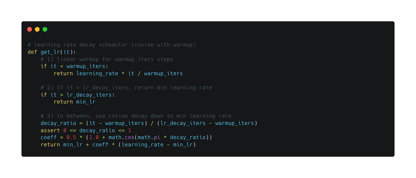
The learning rate. One of the main hyperparameters that we need to think about while pretraining a language model is the learning rate. Typically, we will adopt a schedule for the learning rate during pretraining. An example implementation of a typical learning rate schedule for language model pretraining is shown above. Here, the schedule has a short (linear) warm-up period followed by a (cosine) decay period that lasts for a specified number of iterations; see below.
The training loop. Now that we have done all of the necessary setup, we can finally implement the actual (pre)training loop for our language model; see below.
There may be a few unfamiliar components in the implementation above (e.g., gradient clipping and loss scaling). Most of these changes are related to automatic mixed precision (AMP) training, which is a supported (but not mandatory) component of NanoGPT. Aside from these added details, the above code matches our prior discussion of the pretraining process and uses standard PyTorch syntax.
Closing Thoughts
Reading papers about LLMs is fun and informative, but we can only go so far by just reading. Eventually, we have to implement these ideas if we want to build anything tangible. In this overview, we first learned about the idea of next token prediction and its application to causal language models. Then, we explored a concrete implementation of next token prediction for pretraining and inference with an LLM in PyTorch. Although this implementation is simple compared to some of the massive language models that are explored by current research, it lays a practical foundation that gives us a more concrete understanding of LLMs.
New to the newsletter?
Hi! I’m Cameron R. Wolfe, deep learning Ph.D. and Director of AI at Rebuy. This is the Deep (Learning) Focus newsletter, where I help readers understand AI research via overviews of relevant topics from the ground up. If you like the newsletter, please subscribe, share it, or follow me on Medium, X, and LinkedIn!
Bibliography
[1] Radford, Alec, et al. "Language Models are Unsupervised Multitask Learners."
[2] Radford, Alec, et al. "Improving language understanding by generative pre-training." (2018).
[3] Press, Ofir, and Lior Wolf. "Using the output embedding to improve language models." arXiv preprint arXiv:1608.05859 (2016).
[4] Ott, Myle, et al. "Fully sharded data parallel: faster ai training with fewer gpus." (2021).
[5] Vaswani, Ashish, et al. "Attention is all you need." Advances in neural information processing systems 30 (2017).
[6] Su, Jianlin, et al. "Roformer: Enhanced transformer with rotary position embedding." arXiv preprint arXiv:2104.09864 (2021).
[7] Press, Ofir, Noah A. Smith, and Mike Lewis. "Train short, test long: Attention with linear biases enables input length extrapolation." arXiv preprint arXiv:2108.12409 (2021).
[8] Ouyang, Long, et al. "Training language models to follow instructions with human feedback." Advances in Neural Information Processing Systems 35 (2022): 27730-27744.
[9] Glaese, Amelia, et al. "Improving alignment of dialogue agents via targeted human judgements." arXiv preprint arXiv:2209.14375 (2022).
[10] Yao, Shunyu, et al. "Tree of thoughts: Deliberate problem solving with large language models." arXiv preprint arXiv:2305.10601 (2023).
In fact, I watched the first version of this course during my undergrad, when I was first learning about neural networks. It advanced my understanding significantly and made me capable of implementing a lot of the ideas that I would see in books or papers.
As we will see later, the token embeddings are part of the language model and are trained normally along with the rest of the model’s parameters.
This isn’t always the case. For example, we might be able to support a longer context length but choose to use a shorter context length because a longer context is not necessary for a certain application.
The GPT-2 publication studies multiple sizes of models, the largest of which contains roughly 1.5 billion parameters.
See here for the exact feed-forward network implementation by NanoGPT. The input to the feed-forward model is of size 768 (i.e., size of a single token embedding), while the hidden layer is 4X wider than this.
Notably, the token embedding layer is huge! If we have a vocabulary of V tokens and use d dimensional vectors for each token, this layer has V x d parameters that are learned throughout pretraining. The next token prediction layer has the same exact number of parameters, so tying their weights together is highly beneficial.
We can just think of this as running the training script from multiple terminals at the same time
We specify both rank and local rank. Rank corresponds to a process’ rank among all other processes. Notably, however, we might be running training across several compute nodes (e.g., across several servers, each of which have eight GPUs). Local rank corresponds to the rank of a process on its individual node.









Cameron, by all means, your blog on best LLM/DL blog written on entire Substack (I would rate higher than many paid AI newsletters).
Every blog written by you so neatly written, and anyone can understand complex topics so easily. I’m LLM and Deep Learning beginner but I refer your articles day in day out to learn more. Pls keep it up. Thanks.
Excellent explanation. Thank you.