
Vision Large Language Models (vLLMs)
Teaching LLMs to understand images and videos in addition to text...


After the popularization of text-based large language models (LLMs), one of the most important questions within the research community was how we could extend such powerful models to understand other modalities of data (e.g., images, video or speech). Research on multi-modal LLMs is promising for several reasons:
Improving model capabilities.
Uncovering new sources of training data.
Expanding the scope of problems that LLMs can solve.
Recently, vision-based LLMs—or vLLMs for short, these are LLMs that can ingest images and videos as input in addition to text—have become more popular. For example, most recent OpenAI models support visual inputs, and Meta has released a vision-based variant of LLAMA-3, called LLaMA-3.2 Vision. In this overview, we will aim to understand how vLLMs work from first principles, starting with basic concepts and eventually studying how LLaMA-3.2 Vision is practically implemented. As we will learn, vLLMs—despite their impressive capabilities—are not actually much different than text-based LLMs.
The Building Blocks of vLLMs
To fully understand vLLMs, we need to start from the beginning. In this section, we will cover some of the fundamental concepts used to build these models, including ideas like cross-attention and encoders for images and video. We will (mostly) assume knowledge of the basic concepts behind text-based LLMs, such as a high-level understanding of the transformer architecture. However, readers who are unfamiliar with these concepts can find more details at the link below.

Cross-Attention (and Transformers)

The transformer architecture [8] is used universally within language modeling research. In its original form, the transformer architecture has two components: an encoder and a decoder. As shown above, the encoder and decoder contain repeated blocks of:
Self-attention: transforms each token vector based on the other tokens that are present in the sequence.
Feed-forward transformation: transforms each token vector individually.

The decoder-only transformer is the variant of the transformer architecture that is most commonly used by GPT-style (generative) LLMs. Most vLLMs also utilize a decoder-only architecture, but additional modules are added to the architecture to handle vision-based inputs. Put simply, this architecture is the same as the transformer, but it has no encoder component—hence the name “decoder-only”.
Original decoder. The decoder-only transformer only has masked self-attention and a feed-forward transformation in each of its blocks. However, the decoder from the original transformer architecture has an extra cross-attention module in each of its blocks. Self-attention computes attention over the tokens in a single sequence. In contrast, cross-attention considers two sequences of tokens—the tokens from the encoder and the tokens from the decoder—and computes attention between these two sequences1. By doing this, we allow the decoder to consider the representations produced by the encoder when generating its output! Let’s first try to understand self-attention, then we will cover cross-attention.
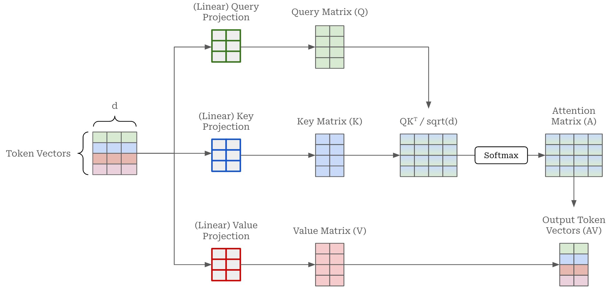
Self-attention at a glance. The input to a self-attention mechanism is a sequence of token vectors. Self-attention forms an output representation for each token by considering all other tokens in the sequence. To do this, the self-attention operation creates three separate linear projections—called the keys, queries, and values—of the token vectors. As shown above, we can then use the keys and queries to compute an attention score between every pair of tokens in the sequence. This attention score captures how important each token is to every other token in the sequence—or how much some token should “pay attention to” another token. We can multiply these attention scores by the values to obtain our final output. A basic implementation of self-attention is provided below2.
| import math | |
| import torch | |
| from torch import nn | |
| import torch.nn.functional as F | |
| class SelfAttention(nn.Module): | |
| def __init__(self, d): | |
| """ | |
| Arguments: | |
| d: size of embedding dimension | |
| """ | |
| super().__init__() | |
| self.d = d | |
| # key, query, value projections for all heads, but in a batch | |
| # output is 3X the dimension because it includes key, query and value | |
| self.c_attn = nn.Linear(d, 3*d, bias=False) | |
| def forward(self, x): | |
| # compute query, key, and value vectors in batch | |
| # split the output into separate query, key, and value tensors | |
| q, k, v = self.c_attn(x).split(self.d, dim=2) | |
| # compute the attention matrix and apply dropout | |
| att = (q @ k.transpose(-2, -1)) * (1.0 / math.sqrt(k.size(-1))) | |
| att = F.softmax(att, dim=-1) | |
| # compute output vectors for each token | |
| y = att @ v | |
| return y |
How does cross-attention work? A schematic depiction of cross-attention is provided below. As we can see, this module is not much different than self-attention. The key difference here is in the initial linear projections used to compute the key, query and value matrices. Instead of computing all three of these matrices by linearly projecting a single sequence of token vectors, we linearly project two different sequences of vectors; see below.

The query matrix is produced by linearly projecting the first sequence, while both key and value matrices are produced by linearly projecting the second sequence. As a result, our attention matrix contains all pairwise attention scores between tokens in the first and second sequence. The length of the sequences need not be equal, and the length of the output will match that of the first sequence.
| import math | |
| import torch | |
| from torch import nn | |
| import torch.nn.functional as F | |
| class CrossAttention(nn.Module): | |
| def __init__(self, d): | |
| """ | |
| Arguments: | |
| d: size of embedding dimension | |
| """ | |
| super().__init__() | |
| self.d = d | |
| # linear projection for producing query matrix | |
| self.w_q = nn.Linear(d, d, bias=False) | |
| # linear projection for producing key / value matrices | |
| self.w_kv = nn.Linear(d, 2*d, bias=False) | |
| def forward(self, x_1, x_2): | |
| # compute query, key, and value matrices | |
| q = self.w_q(x_1) | |
| k, v = self.w_kv(x_2).split(self.d, dim=2) | |
| # compute the attention matrix and apply dropout | |
| att = (q @ k.transpose(-2, -1)) * (1.0 / math.sqrt(k.size(-1))) | |
| att = F.softmax(att, dim=-1) | |
| # compute output vectors for each token in x_1 | |
| y = att @ v | |
| return y |
An implementation of cross-attention is provided above. As outlined in this implementation, we are no longer computing attention scores between tokens within a single sequence. Rather, we are computing inter-sequence attention scores, thus forming a fused representation of the two input sequences.

Application to vLLMs. Our explanation of cross-attention might seem random at this point in the overview. As we will see, however, cross-attention is used constantly in multi-modal LLM research. We can use cross-attention to fuse image representations produced by a vision model into a text-based LLM; see above. In other words, we can incorporate visual information into an LLM as it generates its output, allowing the model to ingest and interpret images (or other modalities of data) as input in addition to just text!
Vision Transformers (ViT) [3]
“We apply a standard Transformer directly to images, with the fewest possible modifications. To do so, we split an image into patches and provide the sequence of linear embeddings of these patches as an input to a Transformer.” - from [3]
Although the transformer (and its many variants like BERT and GPT) were first proposed for natural language processing applications, this influential model architecture has since been expanded to applications in the computer vision domain. The Vision Transformer [3] (or ViT for short) is the most commonly used architecture today. As shown in the figure below, this architecture looks very similar to an encoder-only (BERT-style) transformer architecture. We simply take a sequence of vectors as input and apply a sequence of transformer blocks that contain both i) bidirectional self-attention and ii) a feed-forward transformation.
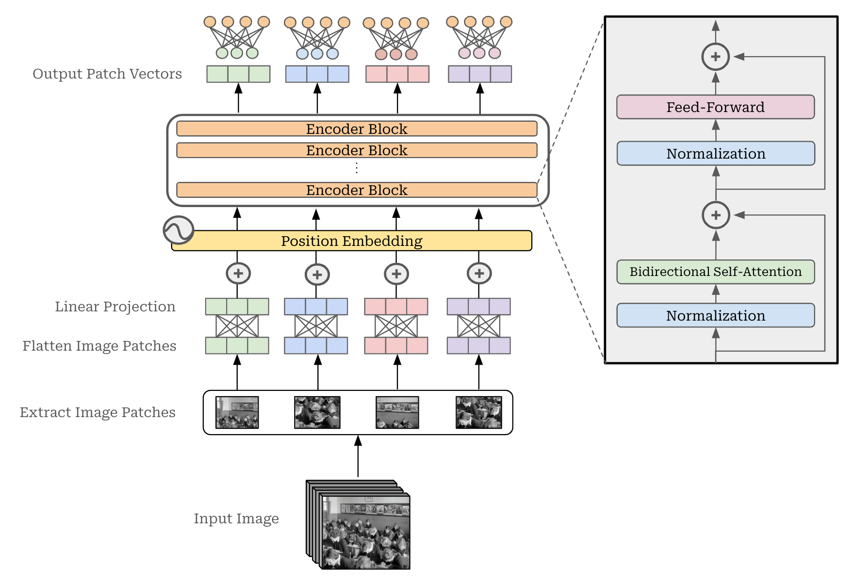
Handling input images. The input for a vision transformer is an image. In order to pass this image as input to our transformer, however, we need to convert the image into a list of vectors—resembling a sequence of textual token vectors. For ViTs, we do this by segmenting an image into a set of patches and flattening each patch into a vector. From here, these vectors may not be of the same size expected by the transformer, so we just linearly project them into the correct dimension.

Similarly to a normal transformer, we add positional embeddings to the vector for each patch. Here, the positional embedding captures the 2D position of each patch within an image. The output of this transformer architecture is a sequence of vectors for each patch that is of the same size as the input. To solve tasks like image classification, we can just add an additional classification module (e.g., a linear layer) to the end of this model, as shown in the figure above.
Why the encoder? We use an encoder-only transformer architecture for the ViT, instead of the decoder-only transformer architecture that is used by most LLMs. The reason for this is that the ViT is not generative. For LLMs, we train the model via next token prediction to generate sequences of text. As a result, we need to use masked self-attention in each transformer layer so that the model cannot look forward in the sequence at future tokens. Otherwise, the model would be able to cheat when predicting the next token! In contrast, the ViT should be able to look at the entire sequence of image patches to form a good representation of the image—we do not need to predict the next patch in this input sequence!
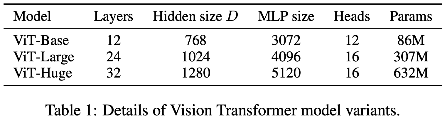
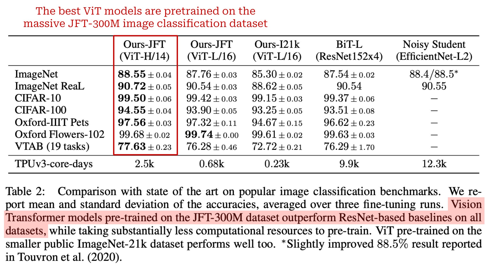
Training ViT. The original ViT model in [3] shares the same architecture as BERT. As shown above, multiple sizes of ViT are trained, the largest of which is ViT-H (or ViT-Huge)—we will see this model again later in the overview. All ViT models are trained using supervised image classification on datasets of varying sizes. When ViTs are trained over small or mid-sized datasets (e.g., ImageNet), they perform comparably to—or slightly worse than—ResNets3 of comparable size. However, ViTs begin to shine when pretrained over much larger datasets (e.g., JFT-300M) and finetuned afterwards on downstream tasks; see below.
Contrastive Language-Image Pre-Training (CLIP) [4]
The standard ViT is trained over a large dataset of supervised image classification examples. These models perform best when pretrained over a massive volume of annotated (usually by humans) data, which is difficult and expensive to obtain. In [4], authors explore an alternative approach that uses image-caption pairs, which are more readily available online, to train a powerful image representation model. This approach is called Contrastive Language-Image Pre-Training (CLIP).

CLIP architecture. The CLIP model is made up of two independent components: an image encoder and a text encoder. Given an image-text pair as input, we pass these inputs separately to their corresponding encoder to get an associated vector representation. The image encoder is a standard ViT model [3], whereas the text encoder is a decoder-only transformer (i.e., a typical GPT-style LLM). CLIP’s text encoder is not used to generate text (at least in [4]), but the authors use a decoder-only architecture to simplify the extension of CLIP to generative applications in the future. A depiction of CLIP’s architecture is provided above.
“The simple pre-training task of predicting which caption goes with which image is an efficient and scalable way to learn image representations from scratch on a dataset of 400 million (image, text) pairs collected from the internet.” - from [4]
Contrastive learning. There are many ways that we could approach training the CLIP model described above. For example, we could classify the images based on the words in the caption [5] or use the LLM component of the architecture to generate captions based on the image [6]. However, these objectives were found in prior work to either perform poorly or cause the model to learn slowly. The key contribution of [4] is the idea of using a simple and efficient training objective— based upon ideas from contrastive learning—to learn from image-text pairs.
More specifically, CLIP is trained using the simple task of classifying the correct caption for an image among a group of candidate captions (i.e., all other captions within a training batch). Practically, this objective is implemented by:
Passing a group of images and textual captions through their respective encoders (i.e., the ViT for images and the LLM for text).
Maximizing the cosine similarity between image and text embeddings (obtained from the encoders) of the true image-caption pairs.
Minimizing the cosine similarity between all other image-caption pairs.
This objective is referred to as a multi-class N-pair (or InfoNCE) loss [7] and is commonly used in the contrastive and metric learning literature.
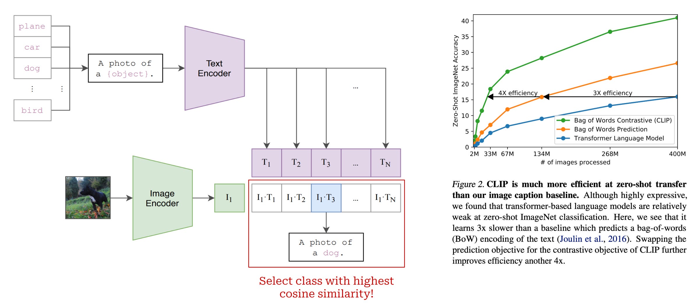
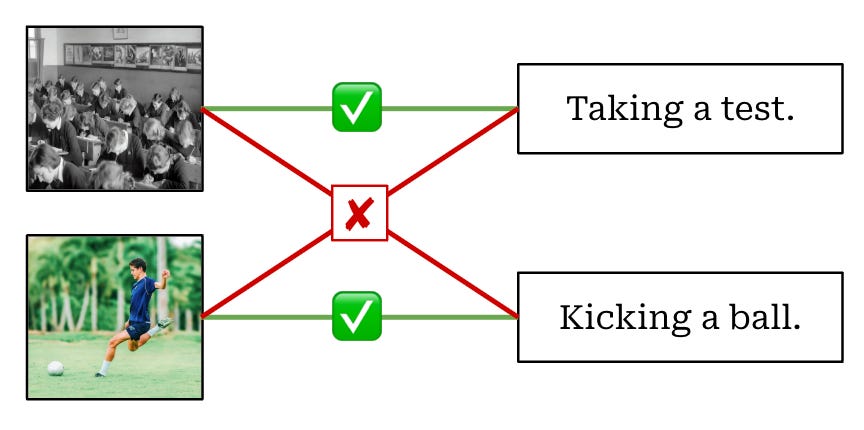
Using CLIP. Although the CLIP model is trained with both an image and text encoder, most of the work we will see in this overview only uses the image encoder from CLIP. The key contribution of CLIP is not the model architecture, but rather the training objective. Using both an image and text encoder allows us to train the image encoder using the contrastive objective described above, which is very efficient (see above) and does not rely on large amounts of supervised data. The CLIP model architecture can be useful as a whole; e.g., we can use it to perform zero-shot image classification as shown above. However, we can also train a CLIP model solely for the purpose of obtaining a high-quality image encoder!
From Images to Videos
To process an image with an LLM, we can simply pass this image to an image encoder (e.g., CLIP) to produce a set of vectors—or embeddings—to represent this image. Then, the LLM can take these embeddings as an additional input (we will cover more details on this later in the overview). However, what if we have access to a video instead of an image? Interestingly, processing video inputs with an LLM is not that much different than processing image inputs—we just need some strategy for converting this video into a set of vectors, similarly to an image!
What is a video? At the simplest level, a video is just an ordered list of images, commonly referred to as “frames”. Usually, images are stored in RGB format. For example, the image in the figure below has three color channels—red, blue and green—as well as a height and width of five. The size of this image is 3 (color channels) × 5 (height) × 5 (width). We can also stack several images into a mini-batch of images, forming a tensor of size batch × 3 × 5 × 5.

The structure of video is not much different—a video is just a collection of ordered frames. When viewed in the correct temporal order, these frames reveal the movement of a scene through time, forming a video. Similar to images, each of these frames are usually represented in RGB-format, and all frames in a video have the same spatial resolution. For example, the video in the figure above has three frames, each with three color channels and a height and width of five, forming a tensor of size 3 (frames) × 3 (color channels) × 5 (height) × 5 (width). We can also create a mini-batch of videos, but we must make sure that each video has the same number of frames—this is usually done by extracting fixed-length “clips” from the video (e.g., with 64 frames).
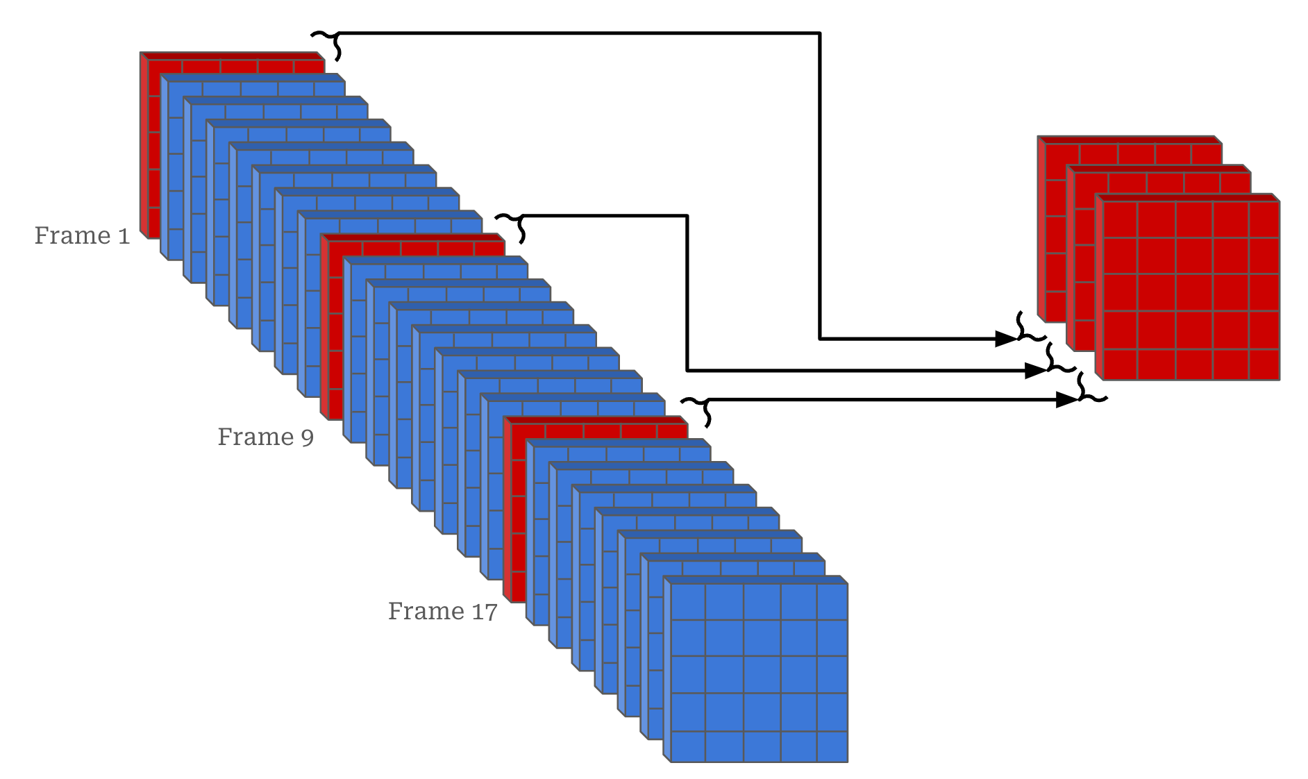
Frame rate. Videos usually have a fixed number of frames per second (FPS) at which they are recorded. For example, 24 FPS is a common frame rate, which means that each second of the video will contain 24 frames. For watching movies or playing video games, having a granular frame rate is important—we do not want to have any visually perceptible gaps between the frames of the video. However, neural networks do not need to process videos at this level of granularity. As shown above, we can save computational costs by sub-sampling the frames within a video; e.g., sampling every eighth frame of a 24 FPS video to simulate 3 FPS.
Encoding a video. Once we have sub-sampled video frames, we can simply treat a video as a set of images! Usually, we pass each video frame independently through an image encoder like CLIP, yielding a corresponding set of vectors to represent each video frame. Then, an LLM can ingest the vectors for these video frames as an additional input, similarly to an image. But, there is still a problem here: the number of vectors produced for the video is large and sometimes unpredictable because the video can be of any length. We need an additional module to aggregate the frame representations for a video into a single, fixed-sized set of vectors!

This is where the Perceiver [9] and Perceiver Resampler [10] come in handy. The perceiver (shown above) is an attention-based neural network architecture that can ingest high-dimensional input—such as large set of vectors of variable size produced from the frames of a video—and output a fixed-size representation based upon this input. Put simply, this means that we can pass all of our video vectors to the Perceiver and it will give us a fixed-size set of vectors in return. Then, we can easily integrate this additional input into an LLM, just like an image!

The Perceiver was originally applied to multi-modal LLMs by Flamingo [10], which proposed the Perceiver Resampler; see above. Flamingo samples video at one FPS (i.e., a single frame from every second of video). Each sub-sampled frame of a video is passed independently through an image encoder4, producing a corresponding image embedding. Before passing these image embeddings to the text-based LLM, however, we pass them through a Perceiver architecture that produces a fixed (64) number of visual token vectors for the video. Then, we integrate these vectors into the LLM using cross-attention as described before.
vLLM Architectures and Training Strategies
We now understand most background concepts relevant to vLLMs. Next, we will use these concepts to build an understanding of vLLMs from the ground up. In this section, we will focus on the architectures and training strategies that are commonly used to create vLLMs. We will keep this discussion conceptual for now, then apply these ideas to implementing a real vLLM in the next section.
vLLM Architecture Variants
The architecture of a vLLM always has two primary components: the LLM backbone and the vision encoder. The LLM backbone is just a standard decoder-only transformer, while the vision encoder is usually a CLIP / ViT model (with an optional Perceiver Resampler if we want to handle video-based inputs). There are two common vLLM architecture variants that fuse these components together: the unified embedding and cross-modality attention architecture. We use the naming scheme for these architectures proposed by Sebastian Raschka in his great overview of vLLMs. Now, let’s learn about how these architectures work.

Token vectors. The LLM backbone takes raw text as input, but this text is first tokenized into a set of discrete tokens and converted into token vectors by retrieving the corresponding embedding for each token from an embedding layer; see above. This set of token vectors can be directly passed as input to the decoder-only transformer architecture. Similarly for images (or videos), we produce a set of token vectors from the vision encoder by passing an image or video through the vision encoder, which returns a set of visual token vectors as output; see below.

Unified embedding. Now, we have a set of text and image (or video) token vectors as input. The first common vLLM architecture simply:
Concatenates these two modalities of vectors together, forming a single sequence of token vectors.
Passes these concatenated vectors directly as input to a decoder-only transformer architecture.
This architecture, referred to as a unified embedding architecture, is depicted in the figure below. Notably, the size of the visual token vectors may not match that of the text token vectors. So, we usually linearly project the token vectors from the vision encoder into the correct dimension prior to concatenation.
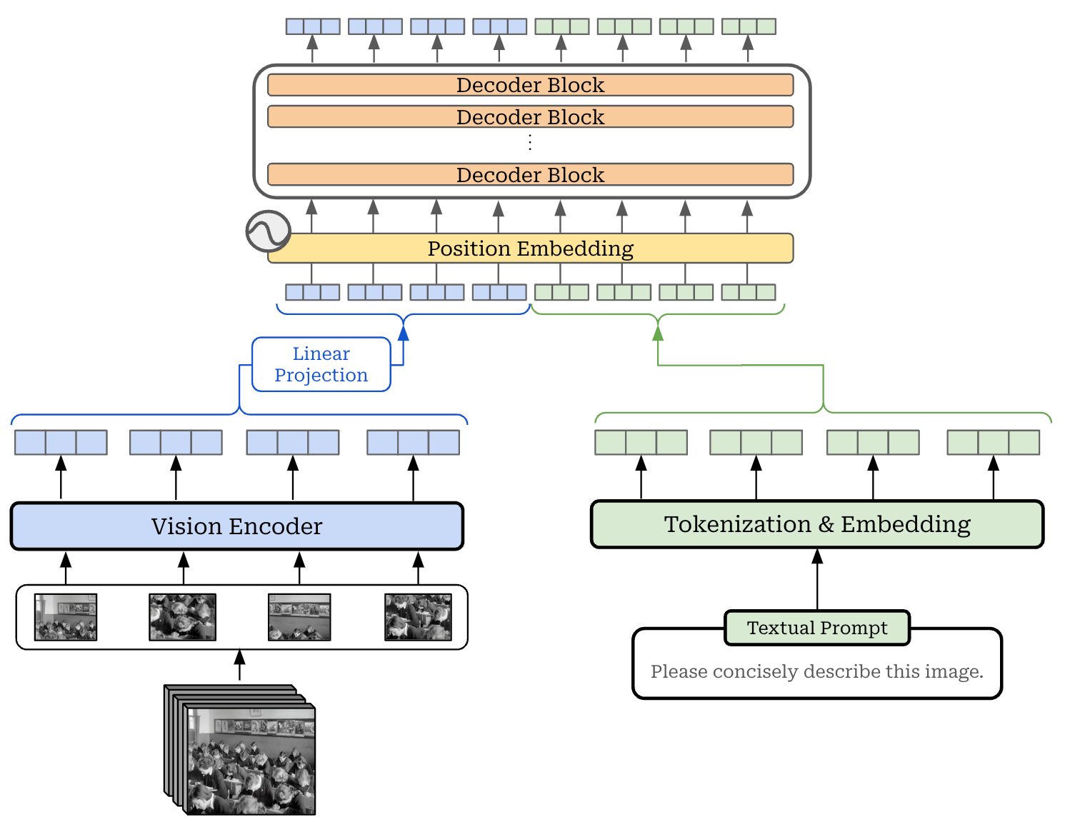
The unified embedding architecture is conceptually simple, but it increases the length of input passed to the LLM, which can cause a significant corresponding increase in computational cost during both training and inference. These visual tokens are passed through every layer of our powerful LLM backbone! Luckily, we can get around this issue by using a slightly different kind of vLLM architecture.
Cross-modality attention. Instead of concatenating text and vision token vectors, we can just pass the text token vectors as input to the LLM. To incorporate vision info, we can add extra cross-attention modules that perform cross-attention between the text and vision token vector into select layers of the LLM—usually every second or fourth layer. This architectural variant is usually referred to as a cross-modality attention architecture; see below for a depiction. Notably, this architecture looks very similar to the original transformer decoder—we just perform cross attention with the image encoder instead of the transformer encoder!
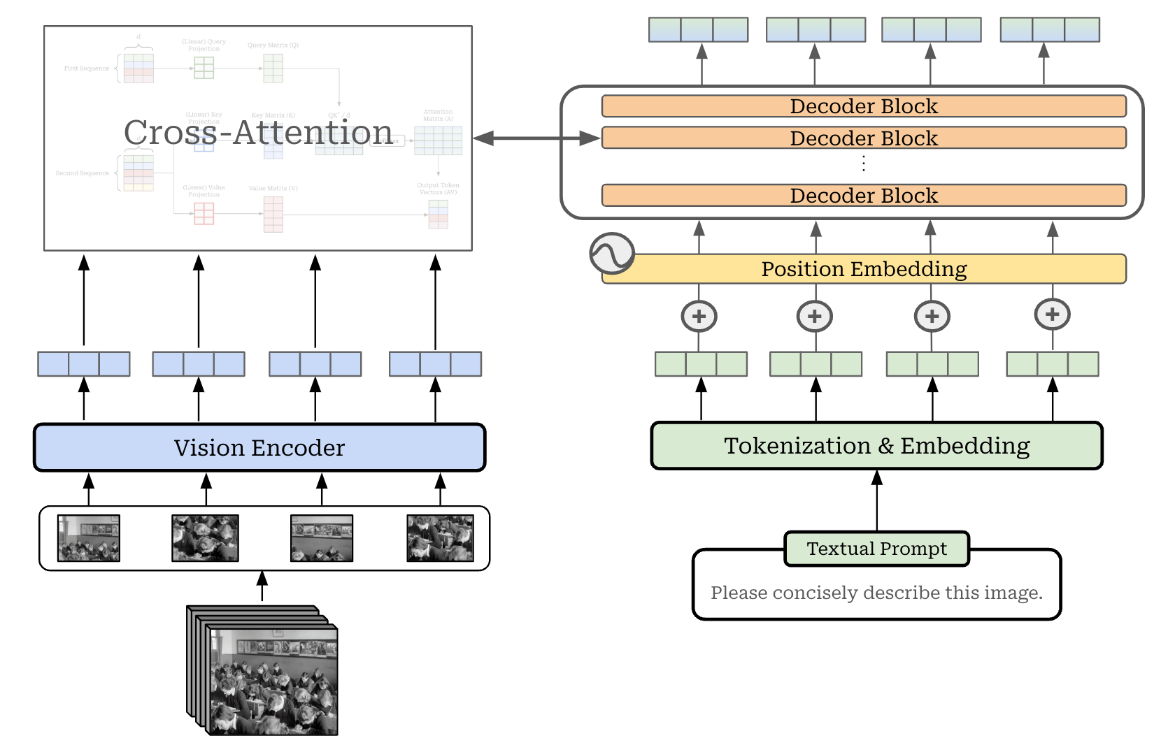
The benefit of this architecture is that we do not increase the length of the input passed to the LLM. Rather, we merge visual information into the LLM by using cross-attention, which is much more computationally efficient. Additionally, the cross-modality attention architecture adds new layers into the model architecture for fusing visual and textual information, rather than relying on the existing layers of the LLM to perform this fusion. For this reason, we can actually leave the LLM backbone fixed during training and only train the added layers, thus ensuring that the LLM’s performance on text-only tasks is not changed at all.
How do we train vLLMs?
In this overview, we will only consider LLMs that can ingest visual inputs—these models still only generate text as output. So, we can train these models similarly to any other LLM: using next-token prediction. Even for the unified embedding architecture, we primarily train the model by predicting textual tokens—we do not typically try to predict visual tokens (i.e., perform next-image prediction).
“The visual encoding of Gemini models is inspired by our own foundational work on Flamingo, CoCa, and PaLI, with the important distinction that the models are multimodal from the beginning and can natively output images using discrete image tokens.” - from [11]
Going beyond the training objective, however, there are several strategies that we can follow for training a vLLM. For example, we could perform native multi-modal training, meaning that we initialize all components of the architecture from scratch and train the model using multi-modal data (i.e., text, images, videos and more) from the beginning; e.g., this approach is used to train Gemini [11].
In practice, however, native multi-modality is complex and difficult. There are many issues that we may encounter when using such approach:
Getting access to a large volume of paired image-and-text data is hard.
Efficient tokenization of visual data at pretraining scale is hard.
Imbalances between modalities can arise; e.g., the model may learn to ignore images because text usually provides enough info for next token prediction.
For these reasons, vLLMs are more frequently trained using a compositional approach. Specifically, this means that we start by pretraining the LLM backbone and the vision encoder independently. Then, we have an additional training phase—we will call this the fusion stage—that combines the text and vision models together into a single vLLM. This approach has several benefits:
The development of text and image models can be parallelized.
Existing text-based LLMs—which are very powerful and advanced—can be used as a starting point for training vLLMs.
A much larger volume of data is available because we can use text-only, vision-only, and paired text-and-vision data for training.
During the fusion phase, we may or may not train the full vLLM architecture. For example, when using a cross-modality attention architecture, we can freeze the LLM backbone during fusion and only train the cross-attention and vision encoder layers. Such an approach is common in the literature because it allows us to start with an existing, text-based LLM and create a corresponding vLLM without making any modifications to the underlying LLM backbone. As we will see, this was the exact approach used to train the LLaMA-3.2 Vision models.
LLaMA-3.2 Vision: Powerful, Open vLLMs
Now that we understand the concepts underlying vLLMs, let’s take a look at a practical case study. The LLaMA-3 [1] LLMs were originally text-only but have since been extended to handle image (and video) inputs. These models are also (mostly) open source5, so we can gain a deep understanding of them by i) studying the details provided in their corresponding technical reports and ii) looking at their code. In this section, we will study in detail how the LLaMA-3 suite of LLMs has been extended to create a corresponding suite of vLLMs.
Extending LLaMA-3 to Images and Video [1]
Proposed in [1], LLaMA-3 is one of the most popular and powerful suites of open-source LLMs. LLaMA-3 models are all dense—meaning they do not use an MoE architecture6—and come in three different sizes: 8B, 70B, and 405B. These models improve upon prior LLaMA-2 models by an order of magnitude—they have a 30× larger context window (128k vs. 4k), use a 30× (15.6T tokens vs. 1.8T tokens) larger dataset, and are trained using 50× the amount of compute.
“We find that Llama 3 delivers comparable quality to leading language models such as GPT-4 on a plethora of tasks… The paper also presents the results of experiments in which we integrate image, video, and speech capabilities into Llama 3 via a compositional approach.” - from [2]
The initial LLaMA-3 models only accept text as input. However, authors include experiments in [1] that incorporate both vision (i.e., image and video) and speech features. We will learn how LLaMA-3 is trained on visual inputs in this section.
Compositional vLLMs. LLaMA-3 follows a compositional approach to creating a multi-modal model. We begin by independently pretraining both a vision encoder and a text-only LLM. Here, the text-only LLM is the text-based LLaMA-3 model, while the vision encoder is a pretrained CLIP model. Adopting a cross-modality attention architecture, we then insert cross-attention layers between these two models and focus on training these extra layers. We will refer to these cross-attention layers as an “image adapter” for convenience. By doing this, the LLM is taught to incorporate additional visual features when generating output.
The vision encoder for LLaMA-3 is based upon the ViT [3] architecture—the 630M parameter ViT-H7 model in particular—and is pretrained via a contrastive objective on 2.5B image-text pairs. In other words, this model is nearly identical to the image encoder component of the CLIP [4] architecture! We create visual features with this model by passing an image through the model and extracting the corresponding embeddings; see below.

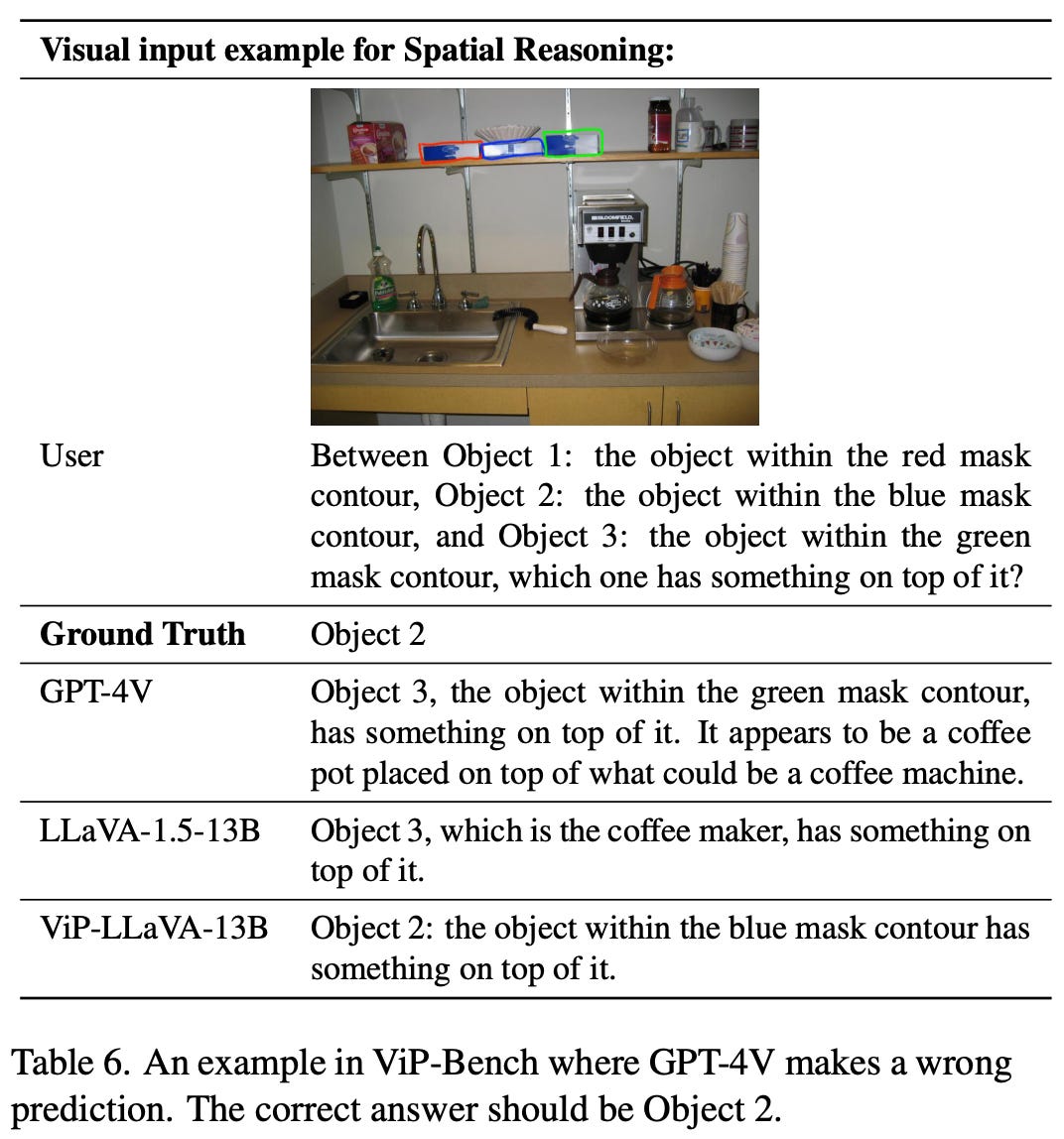
Notably, we know from prior research that image encoders trained with contrastive (CLIP-style) objectives capture semantic information but fail to capture the fine-grained perceptual details of an image. For this reason, any LLM relying upon such visual features may fail to answer questions that require exact localization within an image; see below from an example with GPT-4V. As shown above, this issue is addressed in LLaMA-3 by extracting visual features from several different layers8 of the vision encoder and concatenating them together.
LLaMA-3 also adds several additional self-attention layers after the image encoder and prior to fusion with the LLM—the final image encoder has a total of 850M parameters. This encoder produces 7680-dimensional embeddings for each patch in the input image, and each image has 16 × 16 = 256 patches in total.
“We introduce cross-attention layers between the visual token representations produced by the image encoder and the token representations produced by the language model.” - from [1]
Image adapter. To incorporate features from the image encoder into LLaMA-3, we use a cross-attention-based image adapter. More specifically, cross-attention layers, which compute attention between the textual tokens of the LLM and the image embeddings of the image encoder, are added to every fourth transformer block of the LLM. These cross-attention layers significantly increase the size of the model; e.g., LLaMA-3-405B has ~500B parameters with the image adapter. However, the image adapter allows the LLM to incorporate information from the image encoder into its token representations when generating text.
Video adapter. In addition to images, authors in [1] extend LLaMA-3 to support video inputs. Given that videos are just a sequence of images (or frames), we do not have to significantly modify the existing architecture. The model takes 64 frames as input, each of which is passed through the existing image encoder; see below. To capture the temporal relationship between frames, we use a Perceiver Resampler, which aggregates the representation of 32 consecutive frames into one. Finally, additional video cross-attention layers are added into the LLM.
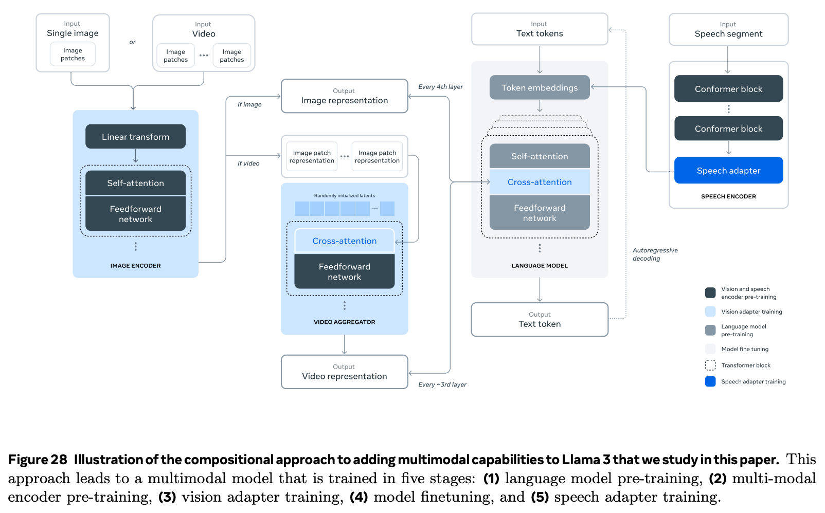
The full architecture of the multi-modal LLaMA-3, including both video and image components, is shown above. Here, we can see that both image and video inputs are first processed via the image encoder, then incorporated into the LLM via cross-attention layers. For videos, we add an extra aggregation module—the Perceiver Resampler—to capture the sequential relationship between video frames.
Pretraining dataset. Both the image encoder and cross-attention layers are trained on a large dataset of image-text pairs. This dataset is filtered to i) remove non-English captions, ii) remove duplicates, iii) remove low-quality data, and iv) maximize diversity (i.e., based on n-gram TF-IDF scores). A very similar process is followed to collect video-text pairs for training the video adapter.
To improve the document understanding capabilities of LLaMA-3, authors in [1] also concatenate OCR output to the end of each textual caption and collect a large number of documents—represented as images—with associated text. Other notable sources of multi-modal training data for LLaMA-3 include:
Visual grounding: noun phrases in the text are linked to bounding boxes / masks in the image that are either overlaid in the image or specified via (normalized) coordinates in the text.
Screenshot parsing: screenshots from HTML code are rendered and the model is asked to predict the code that produced an element—indicated by an overlaid bounding box—in the screenshot.
Question-answer pairs: a large volume of QA data from several sources.
Synthetic captions: images with synthetic captions generated by an early version of LLaMA-3. Authors in [1] observe that synthetic captions tend to be more comprehensive than the original human-written captions.
Synthetic structured images: charts, tables, flowcharts, math equations, and more accompanied by a structured representation (e.g., markdown or LaTeX).
Image adapter training. Prior to training the image adapter, the image encoder is pretrained for several epochs over the image-text pairs in the dataset described above. When training the adapter, the weights of the image encoder are not fixed—they continue to be updated. However, the LLM weights are frozen during this training process. As a result, the LLM backbone of the multi-modal LLaMA-3 model is identical to text-only LLaMA-3, ensuring parity on text-only tasks.
The image adapter is trained in two phases, both of which use a standard language modeling objective applied on the textual caption. In the first phase, all images are resized to a lower resolution to make the training process as efficient as possible. This initial training phase is followed by a second, shorter phase in which we increase the resolution of images and use a smaller (sampled) version of the original dataset that emphasizes the highest quality data. After both training phases are complete, we train the video adapter—beginning with the fully-trained image encoder and adapter—over the video-text dataset using a similar process.
“After pre-training, we fine-tune the model on highly curated multi-modal conversational data to enable chat capabilities. We further implement direct preference optimization (DPO) to boost human evaluation performance and rejection sampling to improve multi-modal reasoning capabilities.” - from [1]
Post training. Similar to the text-based LLaMA-3 model, multi-modal models undergo an entire post training procedure that aligns the model to human preferences, teaches it how to follow instructions, improves its ability to handle conversational inputs and more. Similarly to the text-only LLaMA-3 model, multi-modal models are post trained using a combination of supervised finetuning (SFT), rejection sampling (RS) and direct preference optimization (DPO) applied multiple times sequentially (i.e., in “rounds”). This process is depicted below, and a full overview of post training for LLaMA-3 can be found here.

Unlike when we are training the image encoder and adapter, we do not use the weights of the base LLaMA-3 model for our LLM during post training. Instead, we replace the weights of this base model with those of the LLaMA-3-Instruct model, which has already undergone extensive post training. The dataset for post training is collected from a variety of sources:
Academic datasets that have been converted into conversational format either via a template or by rewriting with an LLM.
Human-annotated datasets that are collected by i) providing a seed image or video and asking the human to write an associated conversation or ii) asking humans to compare model outputs to form preference pairs.
Synthetic datasets collected by giving the text representation (i.e., caption) of an image or video to an LLM and prompting the model to generate related question-answer pairs.
Existing model outputs that have been subtly (but meaningfully) perturbed by an LLM to produce an error, thus forming a preference pair.
Several unique strategies are adopted to optimize the post trained model’s performance. For example, authors train several models—with different hyperparameters—at each stage of post training and obtain the final model by taking the average of these models’ weights. This model merging approach outperforms the best model obtained via a hyperparameter grid search.
LLaMA-3.2: Medium-Sized Vision LLMs [2]

Preliminary experiments with multi-modal LLaMA-3 models were provided in [1], but these models were not officially released until LLaMA-3.2 [2]. The 11B and 90B parameter LLaMA-3.2 Vision models9 were the first LLaMA models to support images as input and have strong capabilities on visual understanding tasks like image captioning and document understanding. Other modalities explored in [1]—such as speech and video—were not included in LLaMA-3.2, and no multi-modal version of the largest (405B parameter) LLaMA-3.1 model is released.
LLaMA-3.2 Vision architecture. The architecture described in [2] for the LLaMA-3.2 Vision models perfectly matches that of the preliminary models outlined in [1]. These models are comprised of:
A pretrained LLM backbone.
A pretrained vision encoder.
Several cross-attention layers between the LLM and vision encoder.
The LLM backbone for LLaMA-3.2 is simply the text-only LLaMA-3.1-8B and LLaMA-3.1-70B models. The vision LLMs are trained in several stages on image-text pairs, but the LLM backbone is not updated during training—we only update the image encoder and adapter layers. As a result, the performance of LLaMA-3.2 Vision models on text-only tasks is left in tact relative to LLaMA-3.1.
Stages of training. As mentioned previously, the LLaMA-3.2 Vision models are trained in multiple stages. First, we must pretrain the LLM backbone and image encoder independently of each other. We then integrate these models together by adding cross attention layers between the two models and pretrain the combined vision model over a large (and noisy) dataset of image-text pairs. Lastly, we train the model further on a medium-sized dataset of higher-quality, enhanced data and perform post training. The post training strategy for vision models includes several rounds of SFT, rejection sampling and DPO (i.e., same as LLaMA-3.1).

Model evaluation. For text-based tasks, the performance of LLaMA-3.2 models is identical to that of LLaMa-3.1—the LLM backbone is left unchanged by the multi-modal pretraining process. However, authors also evaluate the LLaMA-3.2 Vision models across a wide range of visual understanding tasks in [2]; see above. Most notably, these models have strong performance on tasks that involve documents, charts or diagrams. Such an ability is not surprising given that the model is trained over a large number of document-text pairs, as well as synthetic images of charts and tables. On other visual understanding tasks, LLaMA-3.2 continues to perform well and is competitive with several leading foundation models.
LLaMA-3.2 Vision Implementation
Now that we’ve learned about the LLaMA-3.2 Vision models, let’s take a deeper look at their implementation. To do this, we will study their code in torchtune. For simplicity, we will omit some details from the implementation and instead present pseudocode that outlines the key modeling components. However, those who are interested can always read through the full code in torchtune!

Top-level structure. If we look at the primary function for instantiating a LLaMA-3.2 Vision architecture, we will see that the model is—as we should expect—made up of two primary components: an image encoder and an LLM backbone (called the vision decoder above). These two models are combined in a FusionModel. As shown above, we can toggle the trainable components of this FusionModel, which handles setting each model component as trainable or not and passes the output of the vision encoder to the vision decoder in a generic fashion.
# compute the output of the vision encoder
encoder_embed = None
if encoder_input is not None:
    encoder_embed = self.encoder(**encoder_input)

# pass the vision encoder output to the vision decoder
output = self.decoder(
   tokens=tokens,
   mask=mask,
   encoder_input=encoder_embed,
   encoder_mask=encoder_mask,
   input_pos=input_pos,
)
Notably, the input-output structure of the FusionModel is identical to that of a standard transformer decoder in PyTorch10—these two types of models can be used interchangeably. As shown in the code above, we can also supply an encoder mask that allows us to mask any image tokens from chosen textual tokens.
“DeepFusion is a type of fused model architecture where a pretrained encoder is combined with a pretrained decoder (LLM)… This module makes no assumptions on how the encoder and decoder are fused; it simply passes in the encoder embeddings to the decoder and lets the decoder handle any fusion.” - source
The vision encoder used by LLaMA-3.2 Vision is a standard, CLIP-based vision encoder. This encoder passes an input image through CLIP to retrieve a set of image embeddings. From here, we do not directly pass the output of CLIP to the vision decoder—there is an additional VisionProjectionHead module that sits between CLIP and the vision decoder. The implementation is provided below.

This module passes the CLIP embeddings through several extra self-attention layers prior to being ingested by the vision decoder. Additionally, the projection head pulls features from several hidden layers of the CLIP model—instead of just taking the final layer’s output—to ensure that perceptual information is not lost. All of these embeddings are concatenated together and linearly projected so that they match the size of textual token vectors used by the vision decoder.

The vision decoder for LLaMA-3.2 Vision is nearly identical to a standard, text-based LLM; see above. We just modify this architecture to add cross-attention layers to a subset of the layers in the decoder. To do this, a FusionLayer is used, which keeps the parameters of the cross-attention layer and decoder block separate. This way, we can toggle whether each of these components should be trained or not. For example, LLAMA-3.2 trains the cross-attention layers and leaves the LLM backbone fixed throughout the multi-modal training process.
Closing Remarks
The primary takeaway that we should glean from this overview is the fact that vLLMs are not much different than standard, text-based LLMs. We simply add an additional image encoder to this model, as well as some extra layers to fuse the two models together. The fusion between the image encoder and the text-based LLM can be accomplished either via a unified embedding architecture or with cross-modality attention. From here, we can just train this combined model (in multiple phases) over image-text pairs, forming a powerful vLLM. Many variants of vLLMs exist, but the fundamental ideas behind them really are that simple!
New to the newsletter?
Hi! I’m Cameron R. Wolfe, Deep Learning Ph.D. and Machine Learning Scientist at Netflix. This is the Deep (Learning) Focus newsletter, where I help readers better understand important topics in AI research. If you like the newsletter, please subscribe, share it, or follow me on X and LinkedIn!
Bibliography
[1] Grattafiori, Aaron, et al. "The llama 3 herd of models." arXiv preprint arXiv:2407.21783 (2024).
[2] Meta LLaMA Team. “Llama 3.2: Revolutionizing edge AI and vision with open, customizable models” https://ai.meta.com/blog/llama-3-2-connect-2024-vision-edge-mobile-devices/ (2024).
[3] Dosovitskiy, Alexey, et al. "An image is worth 16x16 words: Transformers for image recognition at scale." arXiv preprint arXiv:2010.11929 (2020).
[4] Radford, Alec, et al. "Learning transferable visual models from natural language supervision." International conference on machine learning. PmLR, 2021.
[5] Joulin, Armand, et al. "Learning visual features from large weakly supervised data." Computer Vision–ECCV 2016: 14th European Conference, Amsterdam, The Netherlands, October 11–14, 2016, Proceedings, Part VII 14. Springer International Publishing, 2016.
[6] Desai, Karan, and Justin Johnson. "Virtex: Learning visual representations from textual annotations." Proceedings of the IEEE/CVF conference on computer vision and pattern recognition. 2021.
[7] Sohn, Kihyuk. “Improved deep metric learning with multi-class n-pair loss objective.” Advances in neural information processing systems 29 (2016).
[8] Vaswani, Ashish, et al. "Attention is all you need." Advances in neural information processing systems 30 (2017).
[9] Jaegle, Andrew, et al. "Perceiver: General perception with iterative attention." International conference on machine learning. PMLR, 2021.
[10] Alayrac, Jean-Baptiste, et al. "Flamingo: a visual language model for few-shot learning." Advances in neural information processing systems 35 (2022): 23716-23736.
[11] Team, Gemini, et al. "Gemini: A family of highly capable multimodal models, 2024." arXiv preprint arXiv:2312.11805 (2024).
Obviously, the decoder-only transformer has no encoder component, so the cross attention modules are simply removed from this architecture.
When we compute attention scores, we divide all attention scores by the square root of d, the size of the vectors being used for self-attention. This is called scaled dot product attention, and performing this division helps to improve training stability.
Prior to the proposal of ViTs, the most commonly-used architecture for computer vision tasks was convolutional neural networks (CNNs), or ResNets in particular.
Specifically, Flamingo uses a ResNet architecture to produce image embeddings, but we could also use CLIP (the more commonly-used vision encoder for LLMs).
See this writeup for a deeper overview of the actual definition of open source and different kinds of “open” LLMs that exist.
In [1], authors mention that they avoid using an MoE architecture due to their design principle of maximizing simplicity. MoEs are more complex and difficult to train.
The “H” here just stands for “Huge”. This is the biggest ViT architecture in terms of total parameters explored in [3].
The motivation for this strategy is that different layers of the ViT will capture different kinds of information. For example, the early layers of the model are likely to capture low-level spatial details, while later layers capture semantic information; see this paper.
Lightweight models with 1B and 3B parameters were also released as part of LLaMA-3.2, but these models only support textual input.
Remember, the transformer decoder has the option to provide a sequence of token vectors from an encoder as input by default. In the standard transformer, the encoder is the text encoder from the full encoder-decoder architecture. For LLaMA-3.2 Vision, the encoder is a vision encoder!
Makes such a complex concept approachable! Thank you for taking the time
loved the article
clarifies a lot of my questions, thanks