Beyond NeRFs (Part One)
Increasing NeRF training speed by 100x or more...
This newsletter is sponsored by Rebuy, where AI is being used to build the future of e-commerce personalization. If you like this newsletter, please subscribe, share it, or follow me on twitter. Thank you for your support!
As we have seen in previous overviews, the proposal of Neural Radiance Fields (NeRFs) [4] was a breakthrough in the domain of neural scene representations. Given some images of an underlying scene, we can train a NeRF to generate arbitrary viewpoints of this scene at high resolution. Put simply, NeRFs leverage deep learning to provide photorealistic renderings of 3D scenes.
But, they have a few notable problems. Within this overview, we will focus on two limitations of NeRFs in particular:
Training a NeRF that can accurately render new viewpoints requires many images of the underlying scene.
Performing training (and rendering) with NeRFs is slow.
As a solution to these problems, we will overview two notable extensions of the NeRF methodology: PixelNeRF [1] and InstantNGP [2]. In learning about these methods, we will see that most problems faced by NeRF can be solved by crafting higher-quality input data and leveraging the ability of deep neural networks to generalize learned patterns to new scenarios.
Background
We have recently learned about many different methods for modeling 3D shapes and scenes with deep learning. These overviews have contained several background concepts that will also be useful for understanding the concepts within this overview:
Feed-forward neural networks [link]
Positional embeddings [link]
Signed distance functions [link]
How 3D data is represented [link]
Beyond these concepts, it will also be very useful within this overview to have a working understanding of NeRFs [4]. To build this understanding, I recommend reading my overview on NeRFs below!
Feature Pyramids
Within this post, we will see several instances in which we use deep neural networks to convert an image into a corresponding (pyramid) feature representation. But, some of us might be unfamiliar with this concept. As such, we need to quickly learn about features representations and overview some different variants of this idea we might encounter within deep learning.
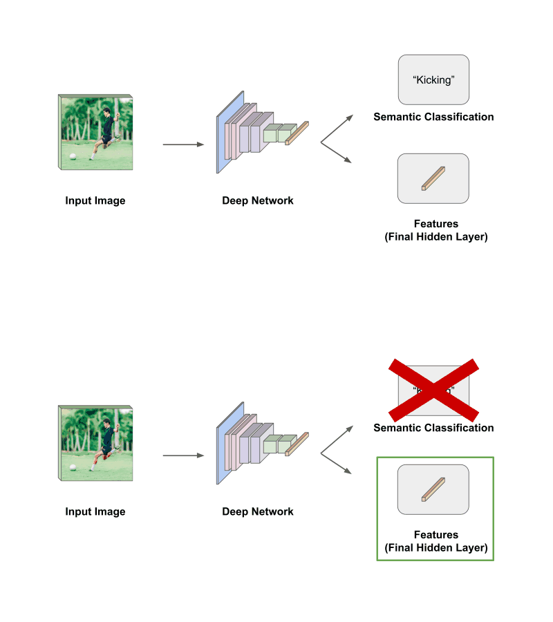
what are features? Before learning about feature pyramids, we need to understand what is meant by the word “features”. Typically, the output of a neural network will be a classification, a set of bounding boxes, a segmentation mask, or something else along these lines. In image classification, for example, we take an image as input, pass it through our neural network, and the final layer of this network is a classification module that converts the hidden state into a vector of class probabilities. Simple enough!
Sometimes, however, we don’t want to perform this last step. Instead, we can just take the final hidden state of the network (before the classification module) and use this vector as a representation of our data; see above. This vector, also referred to as features (or a feature representation), is a compressed representation of the semantic information in our data, and we can use it to perform a variety of tasks (e.g., similarity search).
what is a feature pyramid? Multi-scale (or “pyramid”) strategies are an important, fundamental concept within computer vision. The basic idea is simple. Throughout the layers of a neural network, we occasionally (i) downsample the spatial resolution of our features and (ii) increase the channel dimension. See, for example, the schema of a ResNet-18 [6]. This CNN contains four “sections”, each of which has a progressively higher channel dimension and lower spatial dimension; see below.
One way to extract features from this network is to just use the final hidden representation. But, this representation does not contain much spatial information (i.e., the spatial dimension gets progressively lower in each layer!) compared to earlier layers in the network. This is a problem for dense prediction tasks (e.g., object detection) that are heavily dependent upon spatial info in an image! To fix this, we need to construct a feature pyramid [3].
Put simply, a feature pyramid extracts features from several different layers within a network instead of just using the features from the network’s final layer; see below.
The resulting set of features contains information with varying amounts of spatial and semantic information, as each layer has a varying spatial and channel dimension. Thus, feature pyramids tend to produce image features that are useful for a variety of different tasks. In this overview, we will see feature pyramids used to provide extra input information for a variant of NeRF!
Input Encodings
Sometimes, we have data that we don’t want to input directly into a machine learning model, so we pass an encoded version of this data as input instead. This is a fundamental concept in machine learning. Think about, for example, one-hot encodings of categorical variables. A more sophisticated example would be kernel functions, or functions that we pass our data through (i.e., possibly to make it linearly separable) before giving it to our model. In each of these cases, we are encoding/transforming our input so that it is in a more model-friendly format.
positional encodings. Similarly, when we pass 3D coordinates as input to a NeRF’s feed-forward network, we don’t want to directly use these coordinates as input. Instead, we convert them into a higher-dimensional vector using a positional encoding scheme; see above. This positional encoding scheme is the same exact technique used to add positional information to tokenized inputs within transformers [6]. In NeRFs, positional encodings have been shown to yield significantly improved scene renderings.
learnable embedding layers. There’s one problem with positional encoding schemes—they are fixed. What if we want to learn these encodings instead? One way to do this would be to construct an embedding matrix. Given a function that maps each spatial location to an index in this matrix, we could retrieve the corresponding embedding for each spatial location and use it as input. Then, these embeddings could be trained like normal model parameters!
Publications
Now, we will overview some publications that extend and improve upon NeRFs. In particular, these publications (i) produce high-quality scene representation with fewer images of the scene and (ii) make the training and rendering process of NeRF much faster.
PixelNeRF: Neural Radiance Fields from One or Few Images [1]
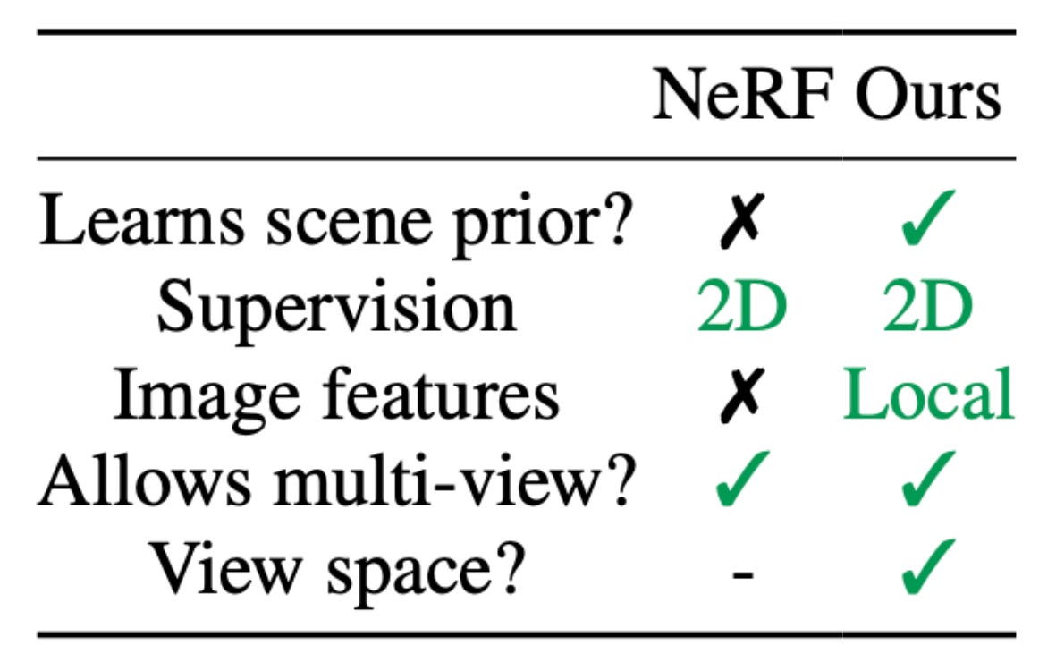
One of the main drawbacks of the original NeRF formulation is that it must be trained and used per-scene. Obtaining a representation for each scene via NeRFs is computationally expensive and requires many posed images of the scene. PixelNeRF [1] aims to mitigate this problem by conditioning a NeRF’s output upon image features—created by a pre-trained deep neural network—from the underlying scene. By using image features as input, PixelNeRF can leverage prior information to generate high-quality scene renderings given only a few images of a scene. Thus, it drastically improves the quality of scene representations given limited data.
method. PixelNeRF is quite similar to the original NeRF formulation. It uses a feed-forward neural network to model a radiance field by predicting color and opaqueness values given a spatial location and viewing direction (that have been converted into positional embeddings) as input. The volume rendering and training procedures are not changed. The main difference between these methods is that pixelNeRF has an additional input component: image features derived from a view of the underlying scene.
PixelNeRF has the ability to consider one or multiple images of the underlying scene as part of its input. Images are first passed through a pre-trained encoder—a feature pyramid R esNet variant[6]—to produce a feature pyramid. From here, we can extract the region of these features corresponding to a specific spatial location (this can be done pretty easily using camera pose information; see Section 4.1 of [1]). Then, we concatenate these extracted features with the corresponding spatial location and viewing direction as input to PixelNeRF’s feed-forward network.
Let’s think about a single forward pass of the feed-forward neural network of PixelNeRF. We consider a single spatial location and viewing direction in this forward pass. If we have access to a single image of the scene, we can include this information by:
Passing the image through the encoder to produce a feature grid.
Obtaining features by extracting the region of this feature pyramid that corresponds to the current spatial location.
Concatenating the spatial, directional, and feature input.
Then, the remaining components of PixelNeRF match the original NeRF formulation; see below.
If multiple images of the underlying scene are available, we just divide PixelNeRF’s feed-forward network into two components. The first component separately processes each image using the procedure described above. Namely, the network performs a separate forward pass by concatenating the features of each image with the same spatial and directional input information.
Each of these forward passes produces an output vector. We can aggregate these vectors by taking their average, then pass this average vector through a few more feed-forward layers to produce the final RGB and opaqueness output; see above. Despite this modified architecture, the training process for PixelNeRF is similar to NeRF and only requires a dataset of scene images.
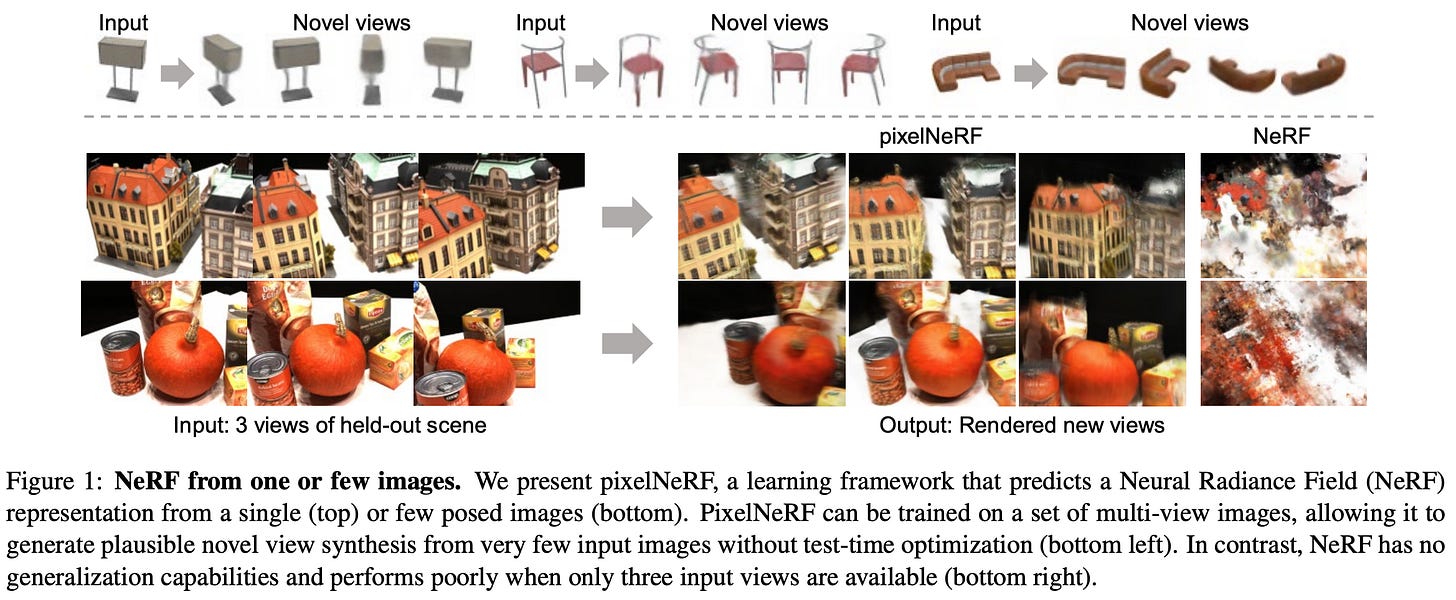
results. PixelNeRF is evaluated on tasks like object and scene view synthesis on ShapeNet, as well as on its ability to represent real-world scenes. First, PixelNeRF is trained to represent objects from a specific ShapeNet class (e.g., chair or car) given one or two images as input (i.e., one or two-shot scenario). In this case, we see that PixelNeRF is better than baselines at reconstructing objects from a few input images; see below.
Plus, PixelNeRF does not perform any test-time optimization, which is not true of baselines like SRNs [5]. Thus, PixelNeRF performs more favorably despite being faster and solving a more difficult problem compared to baselines. When we train PixelNeRF in a category-agnostic fashion (i.e., over 13 object classes in ShapeNet), we see that its performance gains are even more significant! PixelNeRF outperforms baselines across the board on representing this wider set of objects; see below.
When PixelNeRF is evaluated in more complex settings (e.g., unseen categories, multi-object scenes, real images, etc.), we continue to see improved performance. Most notably, PixelNeRF drastically improves upon baselines’ ability to capture multi-object scenes and infer unseen objects at test time; see below.
Taking this to the extreme, PixelNeRF can reconstruct scenes with pretty high fidelity given only three input images of a real-world scene; see below. Such results emphasize the ability of PixelNeRF to model scenes given a limited and noisy input data. NeRF is unable to accurately reconstruct scenes in this regime.
Instant Neural Graphics Primitives with a Multiresolution Hash Encoding [2]
PixelNeRF [1] allows us to recover scene representations from few images of the underlying scene. But, recall that the training process for NeRFs is also slow (i.e., 2 days on a single GPU)! With this in mind, we might ask ourselves: how much faster can we train a NeRF? The proposal of Instant Neural Graphics Primitives (InstantNGP) in [2] shows us that we can train NeRFs a lot faster.
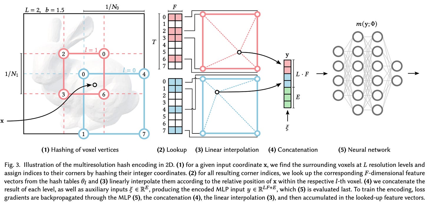
The approach of InstantNGP is similar to NeRF [4]—the only difference lies in how we construct the feed-forward network’s input. Instead of using a positional encoding scheme, we construct a multi-resolution hash table that maps each input coordinate to a trainable feature vector; see above. This approach (i) adds more learnable parameters to the NeRF and (ii) produces rich input representations for each input coordinate, allowing the feed-forward network to be made much smaller. Overall, this approach allows the NeRF training process to be significantly accelerated.
method. The actual approach for constructing and querying the hash table of input features is (unfortunately) more complicated than the simple figure depicted above. Let explore a bit more how exactly input features are handled by InstantNGP [2].
InstantNGP follows a parametric approach to encoding inputs. Unlike NeRFs that use positional embedding functions to map coordinates to fixed, higher-dimensional inputs, InstantNGP learns input features during training. At a high level, this is done by:
Storing input features in an embedding matrix.
Indexing the embedding matrix based on input coordinates.
Updating the features normally via stochastic gradient descent.
Let’s address these components one-by-one. First, we need to create our table of learnable input features that we can index. In [2], input features are stored in a multi-resolution table that contains L levels of features (i.e., just L different embedding matrices). Each level of the table has T features vectors of dimension F (i.e., a matrix of size T x F). Typically, these parameters follow the settings shown below.
Each of the levels is meant to represent 3D space at a different resolution, from N-min (lowest resolution) to N-max (highest resolution). We can think of this as dividing 3D space into voxel grids at different levels of granularity (e.g., N-min will use very large/coarse voxels). By partitioning 3D space in this way, we can determine the voxel in which an input coordinate resides—this will be different for every resolution level. The voxel in which a coordinate resides is then used to map this coordinate to an entry in each level’s embedding matrix.
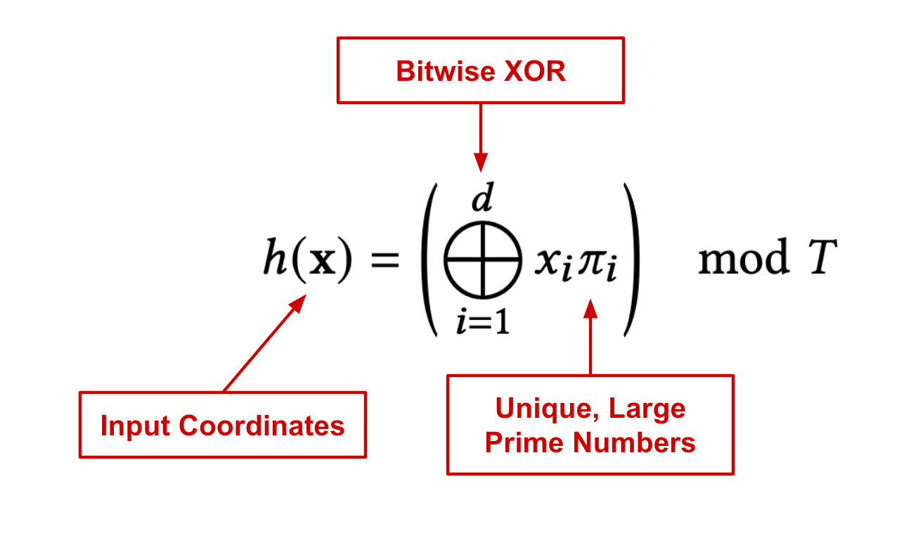
More specifically, authors in [2] use the hash function shown above to map voxel locations (i.e., given by the coordinates of a voxel’s edge) to indices for entries in the embedding matrix at each resolution level. Notably, levels with coarser resolution (i.e., larger voxels) will have fewer hash collisions, meaning that it is less likely for input coordinates at completely different locations to be mapped to the same feature vector.
After we retrieve the corresponding feature vector at each level of resolution, we have multiple feature vectors corresponding to a single input coordinate. To combine these vectors, we linearly interpolate them, where the weights of this interpolation are derived using the relative position of the input coordinate within each level’s voxel. From here, we concatenate these vectors with other input information (e.g., the positionally encoded viewing direction) to form the final input! The full multi-resolution approach in InstantNGP is illustrated within the figure above.
Due to using higher-quality, learnable input features, InstantNGP is able to use much smaller feed-forward networks relative to NeRF while achieving similar results in terms of quality; see above. When these modifications are combined with a more efficient implementation (i.e., fully-fused cuda kernels that minimize bandwidth and wasted operations), the training time for NeRFs can be drastically reduced. In fact, we can use InstantNGP to obtain high-quality scene representations in a matter of seconds.
results. InstantNGP trains a NeRF using a nearly identical setup as proposed in [4], aside from the modified input encoding scheme and smaller feed-forward neural network. Coordinate inputs are encoded using a multi-resolution hash table, while the viewing direction is encoded using normal, positional embeddings.
Using the proposed approach and a faster rendering procedure, authors in [2] find that InstantNGP can train scene representations in seconds and even render scenes at 60 FPS! This is a massive improvement in efficiency relative to NeRF; see above. Notably, InstantNGP becomes competitive with NeRF (which takes hours to train) after only 15 seconds of training!
To determine if this speedup comes from the more efficient cuda implementation or the multi-resolution hash table, the authors do some analysis. They find that the efficient implementation does provide a large speedup, but using the hash table and smaller feed-forward network alone yields a 20X-60X speedup in training NeRFs.
“We replace the hash encoding by the frequency encoding and enlarge the MLP to approximately match the architecture of [NeRF]… This version of our algorithm approaches NeRF’s quality after training for just ∼5 min, yet is outperformed by our full method after training for a much shorter duration (5s–15s), amounting to a 20–60X improvement caused by the hash encoding and smaller MLP.” - from [2]
In certain cases, we do see that baseline methods outperform InstantNGP in scenes that contain complex, view-dependent reflections and non-Lambertian effects. The authors claim this is due to the use of a smaller feed-forward network in [2]; see below.
what else can we use this for? Although we are focusing upon improvements to NeRF, the approach of InstantNGP is quite generic—it can improve the efficiency of a variety of computer graphics primitives (i.e., functions that characterize appearance). For example, InstantNGP is shown in [2] to be effective at:
Generating super-resolution images
Modeling signed distance functions (SDFs)
Performing neural radiance caching
Takeaways
Although NeRFs revolutionized the quality of neural scene representations, we have seen within this overview that there is a lot of room for improvement! NeRFs still take a long time to train and require a lot of training data to work well. Some of the basic takeaways of how we can mitigate these problems are outlined below.
improving sample complexity. In their original form, NeRFs require many input observations of an underlying scene to perform view synthesis. This is mainly because NeRFs are trained separately per-scene, preventing any prior information from being used in generating novel views. PixelNeRF [1] mitigates this problem by adding pre-trained image features as input to NeRF’s feed-forward network. Such an approach allows learned, prior information from other training data to be leveraged. As a result, this method can produce scene representations given only a few images as input!
higher-quality input goes a long way! As shown by InstantNGP [2], the input encoding scheme used by NeRF is incredibly important. Using a richer, learnable encoding scheme for our input allows us to reduce the size of the feed-forward network, which yields significant gains in training and rendering efficiency. In my opinion, such a finding can inspire a lot of future work. Can we find an encoding scheme that’s even better? Are there other types of deep learning models to which this concept can be applied?
limitations. The approaches we have seen in this overview do a lot to solve known limitations of NeRF, but they are not perfect. InstantNGP provides incredible speedups in NeRF training time, but the quality of the resulting scene representations aren’t always the best. InstantNGP struggles to capture complex effects like reflections compared to baselines, revealing that we sacrifice representation quality for faster training.
“On one hand, our method performs best on scenes with high geometric detail… On the other hand, mip-NeRF and NSVF outperform our method on scenes with complex, view-dependent reflections… we attribute this to the much smaller MLP that we necessarily employ to obtain our speedup of several orders of magnitude over these competing implementations.” - from [2]
Additionally, PixelNeRF [1]—due to processing each input image separately in its initial feed-forward component—has a runtime that increases linearly with the number of views used as input. Such a linear dependence can cause both training and rendering to be quite slow. Thus, we can solve some major problems with NeRFs, but it might come at a slight cost!
New to the newsletter?
Hello! I am Cameron R. Wolfe, a research scientist at Alegion and PhD student at Rice University. I study the empirical and theoretical foundations of deep learning.
This is the Deep (Learning) Focus newsletter, where I help readers to build a deeper understanding of topics in deep learning research via understandable overviews of popular papers on that topic. If you like this newsletter, please subscribe, share it with your friends, or follow me on twitter!
Related Posts
iMAP: Modeling 3D Scenes in Real-Time [link]
Understanding NeRFs [link]
Local Light Field Fusion [link]
Scene Representation Networks [link]
Shape Reconstruction with ONets [link]
3D Generative Modeling with DeepSDF [link]
Bibliography
[1] Yu, Alex, et al. "pixelnerf: Neural radiance fields from one or few images." Proceedings of the IEEE/CVF Conference on Computer Vision and Pattern Recognition. 2021.
[2] Müller, Thomas, et al. "Instant neural graphics primitives with a multiresolution hash encoding." ACM Transactions on Graphics (ToG) 41.4 (2022): 1-15.
[3] Lin, Tsung-Yi, et al. "Feature pyramid networks for object detection." Proceedings of the IEEE conference on computer vision and pattern recognition. 2017.
[4] Mildenhall, Ben, et al. "Nerf: Representing scenes as neural radiance fields for view synthesis." Communications of the ACM 65.1 (2021): 99-106.
[5] Sitzmann, Vincent, Michael Zollhöfer, and Gordon Wetzstein. "Scene representation networks: Continuous 3d-structure-aware neural scene representations." Advances in Neural Information Processing Systems 32 (2019).
[6] Vaswani, Ashish, et al. "Attention is all you need." Advances in neural information processing systems 30 (2017).


