Local Light Field Fusion
How to render 3D scenes on a smart phone...
This newsletter is supported by Alegion. At Alegion, I work on a range of problems from online learning to diffusion models. Feel free to check out our data annotation platform or contact me about potential collaboration/opportunities!
If you like this newsletter, please subscribe, share it, or follow me on twitter. Thank you for your support!
By now, we should know that deep learning is a great way to represent 3D scenes and generate new renderings of these scenes from arbitrary viewpoints. The problem with the approaches we have seen so far (e.g., ONets and SRNs [2, 3], however, is that they require many images of the underlying scene to be available to train the model. With this in mind, we might wonder whether it’s possible to obtain a deep learning-based scene representation with fewer samples of the underlying scene. How many images do we actually need to train a high-resolution scene representation?
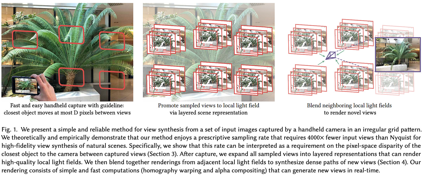
This question was addressed and answered by the Local Light Field Fusion (LLFF) [1] approach for synthesizing scenes in 3D. An extension of light field rendering [4], LLFFs generate scene viewpoints by expanding several sets of existing views into multi-plane image (MPI) representations, then rendering a new viewpoint by blending these representations together. The resulting method:
Accurately models complex scenes and effects like reflections.
Is theoretically shown to reduce the number samples/images required to produce an accurate scene representation.
Plus, LLFFs are prescriptive, meaning that the framework can be used to tell users how many and what type of images are needed to produce an accurate scene representations. Thus, LLFFs are an accurate, deep learning-based methodology for generative modeling of 3D scenes that provide useful, prescriptive insight.
why is this paper important? This post is part of my series on deep learning for 3D shapes and scenes. This area was recently revolutionized by the proposal of NeRF [8]. With a NeRF representation, we can produce an arbitrary number of synthetic viewpoints of a scene or even generate 3D representations of relevant objects; see below. LLFF was proposed slightly before NeRFs, and it is a strong baseline methodology upon which NeRFs improve. The idea of LLFF is helpful context in this domain.
Background
To understand LLFFs, we need to understand a few concepts related to both computer vision and deep learning in general. We will first talk about the concept of light fields, then go over a few deep learning concepts that are used by LLFF.
light fields. A light field represents a 3D scene as rays of light that are directionally flowing through space. Traditionally, we can use light fields to render views of scenes by just (i) sampling a scene’s light field (i.e., capturing images with depth and calibration information) at a bunch of different points and (ii) interpolating between these fields.
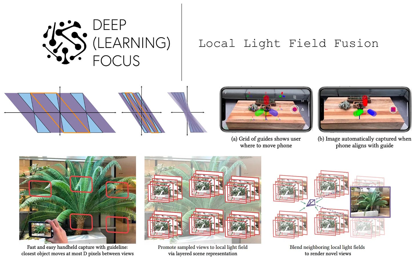
For such a system, we know from research in signal processing how many samples we would have to take to accurately render new views of a scene. The minimum number of samples needed to accurately represent a scene is referred to as the Nyquist rate; see above. Practically, the number of samples required by the Nyquist rate is prohibitive, but research in plenoptic sampling [7] aims to improve sample efficiency and reduce the number of required samples significantly below that of the Nyquist rate.
The inner workings of plenoptic sampling are not important for the purposes of this overview. The main idea that we should take away from this discussion is that authors in [1] extend the idea of plenoptic sampling to enable accurate scene renderings when fewer (and potentially occluded) samples are available; see below.
Beyond its sample efficiency, plenoptic sampling is a theoretical framework that enables prescriptive analysis. Instead of just taking images of a scene and hoping this is enough, we can specifically identify the number and type of images that should be included for training an LLFF by drawing upon this analysis!
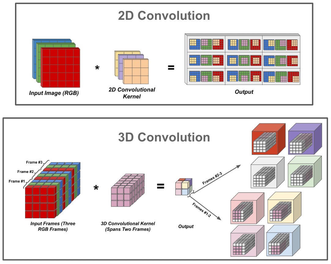
convolutions in 3D. Most of us are probably familiar with 2D convolutions, such as those used within image-based CNNs. However, LLFF actually utilizes 3D convolutions. Why? We will learn more later on, but the basic reason is that the input to our neural network is not just an image or group of images, it has an extra depth dimension. So, we need to perform convolutions in a manner that considers this extra dimension.

3D convolutions accomplish this goal exactly. Namely, instead of just convolving over all spatial dimensions within an input, we convolve over both spatial and depth dimensions. Practically, this adds an extra dimension to our convolutional kernel, and the convolution operation traverses the input both spatially and depth-wise. This process is illustrated in the figure above, where we first spatially convolve over a group of frames, then move on to the next group of frames to perform another spatial convolution.
3D convolutions are commonly used in video deep learning applications. For anyone who is interested in learning more about this topic or the inner workings of 3D convolutions, feel free to check out my overview of deep learning for video at the link below!
perceptual loss. The goal of LLFFs is to produce images that accurately resemble actual, ground truth viewpoints of a scene. To train a system to accomplish this goal, we need an image reconstruction loss that tells us how closely a generated image matches the actual image we are trying to replicate. One option is to compute the L1/L2-norm of the difference between the two images—basically just a mean-squared error loss directly on image pixels.
However, simply measuring pixel differences isn’t the best metric for image similarity; e.g., what if the generated image is just translated one pixel to the right compared to the target? A better approach can be accomplished with a bit of deep learning. In particular we can:
Take a pre-trained deep neural network.
Use this model to embed both images into a feature vector (i.e., the final layer of activations before classification).
Compute the difference between these vectors (e.g., using an L1 or L2-norm)
This approach, called the perceptual loss [5], is a powerful image similarity metric that is used heavily in deep learning research (especially for generative models); see Section 3.3 in [6].
How do LLFFs represent scenes?
“The overall strategy of our method is to use a deep learning pipeline to promote each sampled view to a layered scene representation with D depth layers, and render novel views by blending between renderings from neighboring scene representations.” - from [1]
Starting with some images and camera viewpoint information, LLFFs render novel scene viewpoints using two, distinct steps:
Convert the image into an MPI representation.
Generate a view by blending renderings from nearby MPIs.
what are MPIs? MPIs are a camera-centric representation of 3D space. This means that we consider a specific camera viewpoint, then decompose 3D space from the perspective of this particular viewpoint. In particular, 3D space is decomposed based on three coordinates: x, y, and depth. Then, associated with each of these coordinates is an RGB color and an opaqueness value, denoted as α. See the link below for more details.
generating MPIs. To generate an MPI in LLFF, we need a set of five images, including a reference image and four nearest neighbors in 3D space. Using camera viewpoint information, we can re-project these images into plane sweep volumes (PSVs) with depth D. Here, each depth dimension corresponds to different ranges of depths within a scene from a particular viewpoint.
From here, we can concatenate all of these volumes and pass them through a series of 3D convolutional layers (i.e., a 3D CNN). For each MPI coordinate (i.e., consists of an [x, y] spatial location and a depth), this 3D CNN will output an RGB color and an opacity value α, forming an MPI scene representation; see above. In [1], this is referred to as a “layered scene representation”, due to the different depths represented within the MPI.
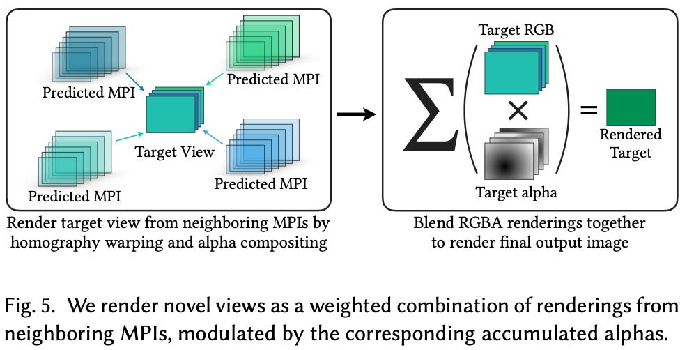
reconstructing a view. Once an MPI is generated for a scene, we still need to take this information and use it to synthesize a novel scene viewpoint. In [1], this is done by rendering multiple MPIs and taking a weighted combination of their results.
In particular, we generate MPIs (using the 3D CNN described above) from multiple sets of images that are close to the desired viewpoint, then use homography warping (i.e., this “warps” each MPI to the desired viewpoint) and alpha compositing (i.e., this combines the different warped MPIs into a single view) to produce an RGB image of the desired viewpoint.
why do we need multiple MPIs? The approach in [1] typically produces two MPIs using different sets of images, then blends these representations into a single scene rendering. This is necessary to remove artifacts within the rendering process and because a single MPI is unlikely to include all the information that’s needed for the new camera pose. For example, what if a portion of the image is occluded in the original viewpoints? Blending multiple MPIs lets us avoid these artifacts and deal with issues like occlusion and limited field of view; see below.
training the LLFF framework. To train the LLFF framework, we use a combination of real and synthetic (e.g., renderings from SUNCG and UnrealCV) data. During each training iteration, we sample two sets of five images (used to create two MPIs) and a single, hold-out viewpoint. We generate an estimate of this held-out viewpoint by following the approach described above, then apply a perceptual loss function [5] that captures how different the outputted viewpoint is from the ground truth.
We can train LLFF end-to-end because all of its components are differentiable. To perform a training iteration, we just need to:
Sample some images.
Generate a predicted viewpoint.
Compute the perceptual loss.
Perform a (stochastic) gradient descent update.
theoretical reduction in required samples. Sampling according to the Nyquist rate is intractable for scene representations because the number of samples required is too high. Luckily, the deep learning-based LLFF approach in [1] is shown theoretically to reduce the number of required samples for an accurate scene representation significantly. In fact, the number of required views for an accurate LLFF reconstruction is shown to be 4,000X below the Nyquist rate empirically; see below.
Using LLFF in practice
LLFFs are evaluated based on their ability to render novel scene viewpoints with limited sampling capability (i.e., far below the Nyquist rate). Within the experimental analysis, one of the first major findings is that blending renderings from multiple MPIs—as opposed to just rendering a view from a single MPI—is quite beneficial. As shown above, this approach improves accuracy and enables non-Lambertian effects (e.g., reflections) to be captured.
LLFF is more capable of modeling complex scenes, both quantitatively and qualitatively, compared to baselines. In particular, LLFF seems to yield much more consistent results when fewer samples of the underlying scene are available, whereas baselines experience a deterioration in performance; see below.
LLFF’s sample efficiency emphasizes the utility of deep learning. Namely, the model can learn implicit prior information from the training data that allows it to better handle ambiguity! To make this point more concrete, let’s consider a case where we have some input views, but this data doesn’t give us all the information we need to produce an accurate, novel view (e.g., maybe some relevant part of the scene is occluded). Because we are using deep learning, our neural network has learned prior patterns from data that allow it to infer a reasonable output in these cases!
To better understand how LLFF compares to baselines, it’s really useful to look at qualitative examples of output. Several examples are provided in the figure above, but these outputs are best viewed as a video so that the smoothness in interpolation between different viewpoints is easily visible. For examples of this, check out the project page for LLFF below!
LLFF on a smart phone. As a practical demonstration of the LLFF framework, authors create a smart phone app for high-quality interpolation between views of a scene. Given a fixed resolution, LLFF can efficiently produce novel scene viewpoints using a reasonable number of scene images. This app instructs the user to capture specific samples of an underlying scene, then renders views from predicted MPIs in real-time using LLFF.
Beyond the quality of LLFF renderings, recall that it is a prescriptive framework, meaning that the authors in [1] provide theory for the number and type of image samples needed to accurately represent a scene. Along these lines, the LLFF app actually guides users to take specific images of the underlying scene. This feature leverages the proposed sampling analysis in [1] to determine needed samples and uses VR overlays to instruct users to capture specific scene viewpoints; see above.
Takeaways
The LLFF framework is quite a bit different from other methods of representing scenes that we have seen so far. It uses a 3D CNN instead of feed-forward networks, comes with theoretical guarantees, and is more related to signal processing than deep learning. Nonetheless, the framework is incredibly interesting, and hopefully the context provided in this overview will make it a bit easier to understand. The major takeaways are as follows.
plenoptic sampling + deep learning. As mentioned throughout this overview, the number of samples required to produce accurate scene representations with LLFF is quite low (especially when compared to the Nyquist rate). Such sample efficiency is partially due to the plenoptic sampling analysis upon which LLFF is based. However, using deep learning allows patterns from training data to be learned and generalized, which has a positive effect on the efficiency and accuracy of resulting scene renderings.
real-time representations. Beyond the quality of viewpoints rendered by LLFF, the method was implemented in a smart phone app that can run in real-time! This practically demonstrates the efficiency of LLFF and shows that it is definitely usable in real world applications. However, performing the necessary preprocessing to render viewpoints with LLFF takes ~10 minutes.
multiple viewpoints. To create the final LLFF result, we generate two MPIs, which are blended together. We could render a scene with a single MPI, but using multiple MPIs is found to create more accurate renderings (i.e., fewer artifacts and missing details). In general, this finding shows us that redundancy is useful for scene representations—useful data that is missing from one viewpoint might be present in another!
limitations. Obviously, the quality of scene representations can always be improved—LLFFs are not perfect. Beyond this simple observation, one potential limitation of LLFF is that, to produce an output, we need to provide several images as input (e.g., experiments in [1] require ten input images for each output). Comparatively, models like SRNs [3] are trained over images of an underlying scene, but they do not necessarily require that these images be present at inference time!
New to the newsletter?
Hello! I am Cameron R. Wolfe, a research scientist at Alegion and PhD student at Rice University. I study the empirical and theoretical foundations of deep learning.
This is the Deep (Learning) Focus newsletter, where I help readers to build a deeper understanding of topics in deep learning research via series of short, focused overviews of popular papers on that topic. Each overview contains explanations of all relevant background information or context. A new topic is chosen (roughly) every month, and I overview two papers each week (on Monday and Thursday). If you like this newsletter, please subscribe, share it with your friends, or follow me on twitter!
Bibliography
[1] Mildenhall, Ben, et al. "Local light field fusion: Practical view synthesis with prescriptive sampling guidelines." ACM Transactions on Graphics (TOG) 38.4 (2019): 1-14.
[2] Mescheder, Lars, et al. "Occupancy networks: Learning 3d reconstruction in function space." Proceedings of the IEEE/CVF conference on computer vision and pattern recognition. 2019.
[3] Sitzmann, Vincent, Michael Zollhöfer, and Gordon Wetzstein. "Scene representation networks: Continuous 3d-structure-aware neural scene representations." Advances in Neural Information Processing Systems 32 (2019).
[4] Levoy, Marc, and Pat Hanrahan. "Light field rendering." Proceedings of the 23rd annual conference on Computer graphics and interactive techniques. 199.
[5] Dosovitskiy, Alexey, and Thomas Brox. "Generating images with perceptual similarity metrics based on deep networks." Advances in neural information processing systems 29 (2016).
[6] Chen, Qifeng, and Vladlen Koltun. "Photographic image synthesis with cascaded refinement networks." Proceedings of the IEEE international conference on computer vision. 2017.
[7] Chai, Jin-Xiang, et al. "Plenoptic sampling." Proceedings of the 27th annual conference on Computer graphics and interactive techniques. 2000.
[8] Mildenhall, Ben, et al. "Nerf: Representing scenes as neural radiance fields for view synthesis." Communications of the ACM 65.1 (2021): 99-106.


