The Best Learning Rate Schedules
Practical and powerful tips for setting the learning rate...
This newsletter is supported by Alegion. As a research scientist at Alegion, I work on a range of problems from online learning to diffusion models. Feel free to check out our data annotation platform or contact me about potential collaboration/opportunities!
Welcome to the Deep (Learning) Focus newsletter. Each issue picks a single topic in deep learning research and comprehensively overviews related research. Feel free to subscribe to the newsletter, share it, or follow me on twitter if you enjoy it!
Anybody that has trained a neural network knows that properly setting the learning rate during training is a pivotal aspect of getting the neural network to perform well. Additionally, the learning rate is typically varied along the training trajectory according to some learning rate schedule. The choice of this schedule also has a large impact on the quality of training.
Most practitioners adopt a few, widely-used strategies for the learning rate schedule during training; e.g., step decay or cosine annealing. Many of these schedules are curated for a particular benchmark, where they have been determined empirically to maximize test accuracy after years of research. But, these strategies often fail to generalize to other experimental settings, raising an important question: what are the most consistent and useful learning rate schedules for training neural networks?
Within this overview, we will look at recent research into various learning rate schedules that can be used to train neural networks. Such research has discovered numerous strategies for the learning rate that are both highly effective and easy to use; e.g., cyclical or triangular learning rate schedules. By studying these methods, we will arrive at several practical takeaways, providing simple tricks that can be immediately applied to improving neural network training.
To supplement this overview, I have implemented the main learning rate schedules that we will explore within a repository found here. These code examples are somewhat minimal, but they are sufficient to implement any of the learning rate schedules discussed in this overview without much effort.
Neural Network Training and the Learning Rate
In a supervised learning setting, the goal of neural network training is to produce a neural network that, given some data as input, can predict the ground truth label associated with that data. One example of this would be training a neural network to correctly predict whether an image contains a cat or a dog based upon a large dataset of labeled images of cats and dogs.
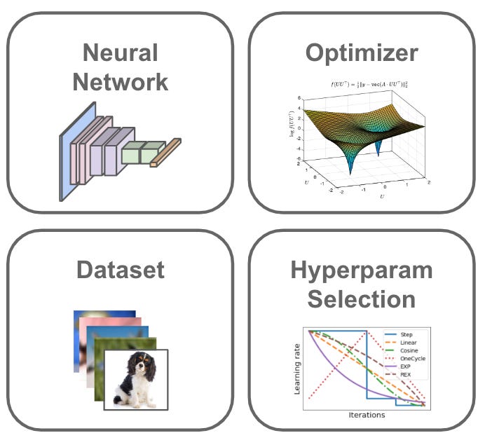
The basic components of neural network training, depicted above, are as follows:
Neural Network: takes some data as input and transforms this data based on its internal parameters/weights to produce some output.
Dataset: a large set of examples of input-output data pairs (e.g., images and their corresponding classifications).
Optimizer: used to update the neural network’s internal parameters such that its predictions become more accurate.
Hyperparameters: external parameters that are set by the deep learning practitioner to control relevant details of the training process.
Usually, a neural network begins training with all of its parameters randomly initialized. To learn more meaningful parameters, the neural network is shown samples of data from the dataset. For each of these samples, the neural network attempts to predict the correct output, then the optimizer updates the neural network’s parameters to improve this prediction.
This process of updating the neural network’s parameters such that it can better match the known outputs within a dataset is referred to as training. The process repeats iteratively, typically until the neural network has looped over the entire dataset – referred to as an epoch of training – multiple times.
Although this description of neural network training is not comprehensive, it should provide enough intuition to make it through this overview. Many extensive tutorials on neural network training exist online. My favorite tutorial by-far is from the “Practical Deep Learning for Coders” course by Jeremy Howard and fast.ai; see the link to the video below.
What are hyperparameters?
Model parameters are updated by the optimizer during training. Hyperparameters, in contrast, are “extra” parameters that we, the deep learning practitioner, have control over. But, what can we actually control with hyperparameters? One common hyperparameter, which is relevant to this overview, is the learning rate.
what is the learning rate? Put simply, each time the optimizer updates the neural network’s parameters, the learning rate controls the size of this update. Should we update the parameters a lot, a little bit, or somewhere in the middle? We make this choice by setting the learning rate.
selecting a good learning rate. Setting the learning rate is one of the most important aspects of training a neural network. If we choose a value that is too large, training will diverge. On the other hand, a learning rate that is too small can yield poor performance and slow training. We must choose a learning rate that is large enough to provide regularization benefits to the training process and converge quickly, while not being too large such that the training process becomes unstable.
Choosing good hyperparameters
Hyperparameters like the learning rate are typically selected using a simple approach called grid search. The basic idea is to:
Define a range of potential values for each hyperparameter
Select a discrete set of values to test within this range
Test all combinations of possible hyperparameter values
Choose the best hyperparameter setting based on validation set performance
Grid search is a simple, exhaustive search for the best hyperparameters. See the illustration below for an example of grid search over potential learning rate values.
A similar approach can be applied to many hyperparameters at once by following a similar approach and testing all possible combinations of hyperparameter values.
Grid search is computationally inefficient, as it requires the neural network to be retrained for each hyperparameter setting. To avoid this cost, many deep learning practitioners adopt a “guess and check” approach of trying several hyperparameters within a reasonable range and seeing what works. Alternative methodologies for selecting optimal hyperparameters have been proposed [5], but grid search or guess and check procedures are commonly used due to their simplicity.
Learning rate scheduling
After selecting a learning rate, we typically should not maintain this same learning rate throughout the entire training process. Rather, conventional wisdom suggests that we should (i) select an initial learning rate, then (ii) decay this learning rate throughout the training process [1]. The function by which we perform this decay is referred to as the learning rate schedule.
Many different learning rate schedules have been proposed over the years; e.g., step decay (i.e., decaying the learning rate by 10X a few times during training) or cosine annealing; see the figure below. In this overview, we will explore a number of recently proposed schedules that perform especially well.
adaptive optimization techniques. Neural network training according to stochastic gradient descent (SGD) selects a single, global learning rate that is used for updating all model parameters. Beyond SGD, adaptive optimization techniques have been proposed (e.g., RMSProp or Adam [6]), which use training statistics to dynamically adjust the learning rate used for each of a model’s parameters. Most of the results outlined within this overview apply to both adaptive and SGD-style optimizers.
Publications
In this section, we will see several examples of recently proposed learning rate schedules. These include strategies like cyclical or triangular learning rates, as well as different profiles for learning rate decay. The optimal learning rate strategy is highly-dependent upon the domain and experimental settings, but we will see that several high-level takeaways can be drawn by studying the empirical results of many different learning rate strategies.
Cyclical Learning Rates for Training Neural Networks [1]
Authors in [1] propose a new method for handling the learning rate during neural network training: cyclically varying it between a minimum and a maximum value according to a smooth schedule. Prior to this work, most practitioners adopted the popular strategy of (i) setting the learning rate to an initially large value, then (ii) decaying the learning rate as training proceeds.
In [1], we throw away this rule-of-thumb in favor of a cyclical strategy. Cycling the learning rate in this way is somewhat counterintuitive — increasing the learning rate during training damages model performance, right? Despite temporarily degrading network performance as the learning rate increases, cyclical learning rate schedules actually provide a lot of benefits over the full course of training, as we will see in [1].
Cyclical learning rates introduce three new hyperparameters: stepsize, minimum learning rate, and maximum learning rate. The resulting schedule is “triangular”, meaning that the learning rate is increased/decreased in adjacent cycles; see above. The stepsize can be set somewhere between 2-10 training epochs, while the range for the learning rate is typically discovered via a learning rate range test (see Section 3.3 of [1]).
Increasing the learning rate temporarily degrades model performance. Once the learning rate has decayed again, however, the model’s performance will recover and improve. With this in mind, we see in the experimental results of [1] that models trained with cyclical learning rates follow a cyclical pattern in their performance. Model performance peaks at the end of each cycle (i.e., when the learning rate decays back to the minimum value) and becomes somewhat worse at intermediate stages of the cycle (i.e., when the learning rate is increased); see below.
The results in [1] reveal that cyclical learning rates benefit model performance over the course of training. Models trained via cyclical learning rates reach higher levels of performance faster than models trained with other learning rate strategies; see the figure below. In other words, the anytime performance of models trained with cyclical learning rates is really good!
In larger-scale experiments on ImageNet, cyclical learning rates still provide benefits, though they are a bit less pronounced.
SGDR: Stochastic Gradient Descent with Warm Restarts [2]
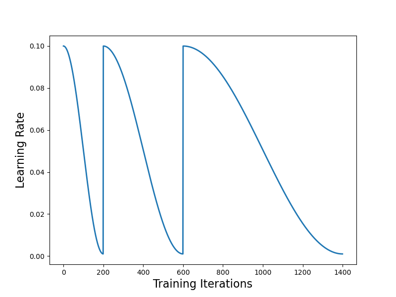
The authors in [2] propose a simple restarting technique for the learning rate, called stochastic gradient descent with restarts (SGDR), in which the learning rate is periodically reset to its original value and scheduled to decrease. This technique employs the following steps:
Decay the learning rate according to some fixed schedule
Reset the learning rate to its original value after the end of the decay schedule
Return to step #1 (i.e., decay the learning rate again)
A depiction of different schedules that follow this strategy is provided below.
We can notice a few things about the schedules above. First, a cosine decay schedule is always used in [2] (the plot’s y-axis is in log scale). Additionally, the length of each decay schedule may increase as training progresses. Concretely, authors in [2] define the length of the first decay cycle as T_0, then multiply this length by T_mult during each successive decay cycle; see below for a depiction.
To follow the terminology of [1], the stepsize of SGDR may increase after each cycle. Unlike [1], however, SGDR is not triangular (i.e., each cycle just decays the learning rate).
In experiments on CIFAR10/100, we can see that SGDR learning rate schedules yield good model performance more quickly than step decay schedules — SGDR has good anytime performance. The models obtained after each decay cycle perform well and continue to get better in successive decay cycles.
Going beyond these initial results, we can study model ensembles formed by taking “snapshots” at the end of each decay cycle. In particular, we can save a copy of the model’s state after each decay cycle within an SGDR schedule. Then, after training is complete, we can average the predictions of each of these models at inference time, forming an ensemble/group of models; see the link below for more details on the idea of ensembles.
By forming model ensembles in this way, we can achieve pretty significant reductions in test error on CIFAR10; see below.
Additionally, the snapshots from SGDR seem to provide a set of models with diverse predictions. Forming an ensemble in this way actually outperforms the normal approach of adding independent, fully-trained models into an ensemble.
Super-Convergence: Very Fast Training of Neural Networks Using Large Learning Rates [3]
The authors in [3] study an interesting approach for training neural networks that allows the speed of training to be increased by an order of magnitude. The basic approach — originally outlined in [8] — is to perform a single, triangular learning rate cycle with a large maximum learning rate, then allow the learning rate to decay below the minimum value of this cycle at the end of training; see below for an illustration.
In addition, the momentum is cycled in the opposite direction of the learning rate (typically in the range [0.85, 0.95]). This approach of jointly cycling the learning rate and momentum is referred to as “1cycle”. The authors in [3] show that it can be used to achieve “super-convergence” (i.e., extremely fast convergence to a high-performing solution).
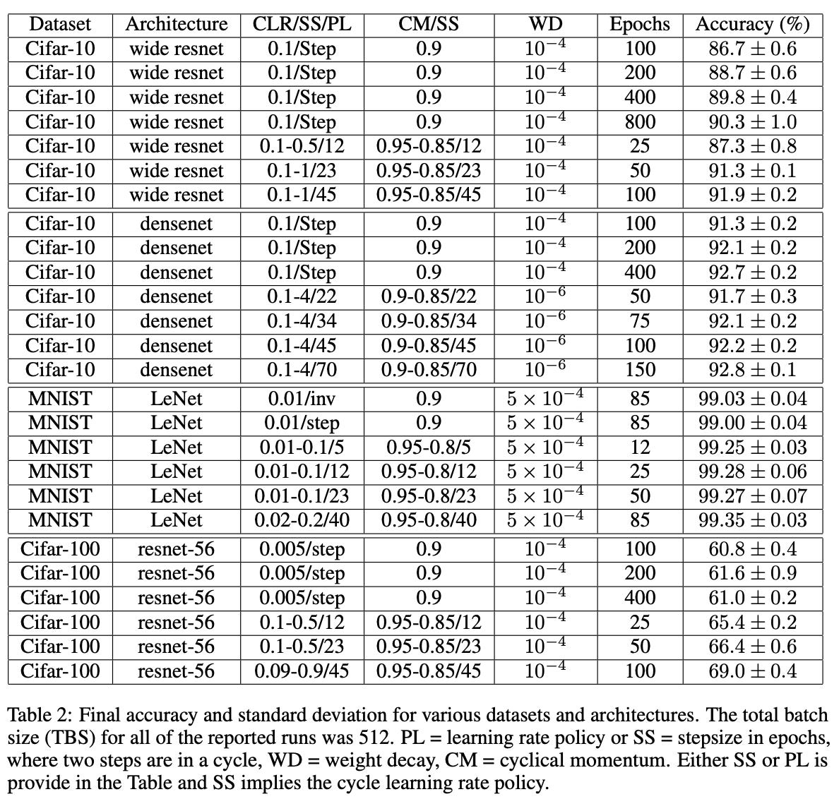
For example, we see in experiments on CIFAR10 that 1cycle can achieve better performance than baseline learning rate strategies with 8X fewer training iterations. Using different 1cycle step sizes can yield even further speedups in training, though the accuracy level varies depending on the step size.
We can observe similar results on a few different architectures and datasets. See the table below, where 1cycle again yields good performance in a surprisingly small number of training epochs.
Currently, it is not clear whether super-convergence is achievable in a wide number of experimental settings, as experiments provided in [3] are somewhat limited in scale and variety. Nonetheless, we can probably all agree that the super-convergence phenomenon is quite interesting. In fact, the result was so interesting that it was even popularized and studied in depth by the fast.ai community.
REX: Revisiting Budgeted Training with an Improved Schedule [4]
Within [4], authors (including myself) consider the problem of properly scheduling the learning rate given different budget regimes (i.e., small, medium, or large number of training epochs). You might be thinking: why would we consider this setting? Well, oftentimes the optimal number of training epochs is not known ahead of time. Plus, we might be working with a fixed monetary budget that limits the number of training epochs we can perform.
To find the best budget-agnostic learning rate schedules, we must first define the space of possible learning rate schedules that will be considered. In [4], we do this by decomposing a learning rate schedule into two components:
Profile: the function according to which the learning rate is varied throughout training.
Sampling Rate: the frequency with which the learning rate is updated according to the chosen profile.
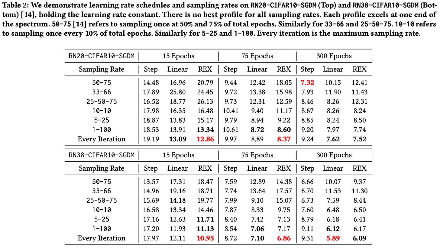
Such a decomposition can be used to describe nearly all fixed-structure learning rate schedules. Different profile and sampling rate combinations are depicted below. Higher sampling rates cause the schedule to match the underlying profile more closely.
Authors in [4] consider learning rate schedules formed with different sampling rates and three function profiles — exponential (i.e., produces step schedules), linear, and REX (i.e., a novel profile defined in [4]); see the figure above.
From here, the authors train a Resnet20/38 on CIFAR10 with different sampling rate and profile combinations. In these experiments, we see that step decay schedules (i.e., exponential profile with a low sampling rate) only perform well given a low sampling rate and many training epochs. REX schedules with every iteration sampling perform well in all different epoch settings.
Prior work indicated that a linear decay schedule is best for low-budget training settings (i.e., training with fewer epochs) [9]. In [4], we can see that REX is actually a better choice, as it avoids decaying the learning rate too early during training.
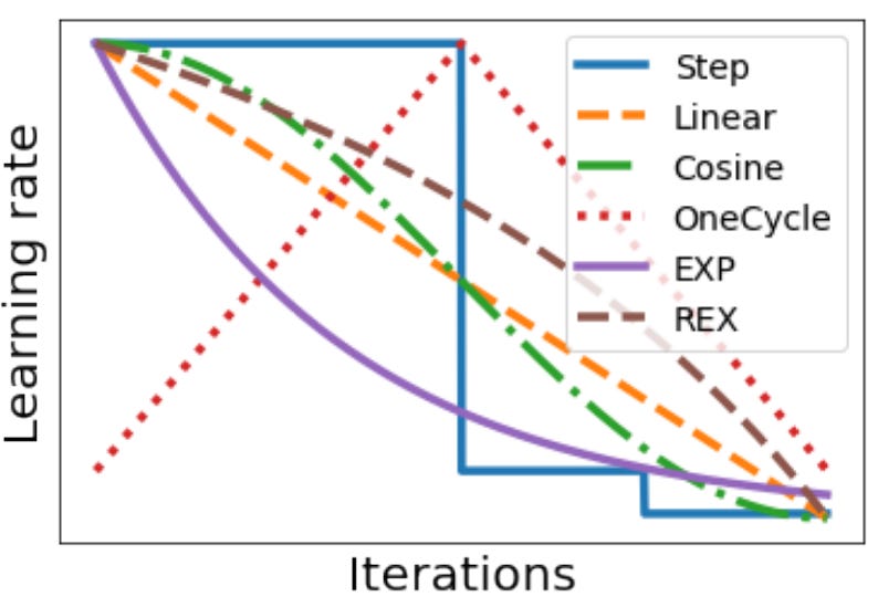
From here, authors in [4] consider a variety of popular learning rate schedules, as shown in the figure below.
These schedules are tested across a variety of domains and training epoch budgets. When the performance is aggregated across all experiments, we get the results shown below.
Immediately, we see that REX achieves shockingly consistent performance across different budget regimes and experimental domains. No other learning rate schedule achieves close to the same ratio of top-1/3 finishes across experiments, revealing that REX is a good domain/budget-agnostic learning rate schedule.
Beyond the consistency of REX, these results teach us something more general: commonly-used learning rate strategies don’t generalize well across experimental settings. Each schedule (even REX, though to a lesser degree) performs best in only a small number of cases, revealing that selecting the proper learning rate strategy for any particular setting is incredibly important.
Takeaways
Properly handling the learning rate is arguably the most important aspect of neural network training. Within this overview, we have learned about several practical learning rate schedules for training deep networks. Studying this line of work provides takeaways that are simple to understand, easy to implement, and highly effective. Some of these basic takeaways are outlined below.
Choose a good learning rate. Properly setting the learning rate is one of the most important aspects of training a high-performing neural network. Choosing a poor initial learning rate or using the wrong learning rate schedule drastically deteriorates model performance.
The “default” schedule isn’t always best. Many experimental settings have a “default” learning rate schedule that we tend to adopt without much thought; e.g., step decay schedules for training CNNs for image classification. We should be aware that the performance of these schedules may deteriorate drastically as experimental settings change; e.g., for budgeted settings, REX-based schedules significantly outperform step decay. As practitioners, we should always be mindful of our chosen learning rate schedule to truly maximize our model’s performance.
Cyclical schedules are awesome. Cyclical or triangular learning rate schedules (e.g., as in [2] or [3]) are really useful because:
They often match or exceed state-of-the-art performance
They have good anytime performance
Using cyclical learning rate strategies, models reach their best performance at the end of each decay cycle. We can simply continue training for any given number of cycles until we are happy with the network’s performance. The optimal amount of training need not be known a priori, which is often useful in practice.
There’s a lot to explore out there. Although learning rate strategies have been widely studied, it seems like there is still more out there to be discovered. For example, we have seen that adopting alternative decay profiles benefits budgeted settings [4] and cyclical strategies may even be used to achieve super-convergence in some cases [3]. My question is: what more can be discovered? It seems like there are really interesting strategies (e.g., fractal learning rates [7]) that are yet to be explored.
Software resources
As a supplement to this overview, I created a lightweight code repository for reproducing some of the different learning rate schedules, which includes:
Functions to generate different decay profiles
Functions for adjusting the learning rate/momentum in PyTorch optimizers
Working examples for common learning rate schedules we have seen in this overview
Although a bit minimal, this code provides everything that’s needed to implement and use any of the learning rate strategies we have studied so far. A link to the repository is provided below.
If you’re not interested in using this code, you can also use the learning rate schedulers directly implemented within PyTorch.
New to the newsletter?
Hello! I am Cameron R. Wolfe, a research scientist at Alegion and PhD student at Rice University studying the empirical and theoretical foundations of deep learning. This is the Deep (Learning) Focus newsletter, where I pick a single, bi-weekly topic in deep learning research, provide an understanding of relevant background information, then overview a handful of popular papers on the topic. If you like this newsletter, please subscribe, share it with your friends, or follow me on twitter!
Bibliography
[1] Smith, Leslie N. "Cyclical learning rates for training neural networks." 2017 IEEE winter conference on applications of computer vision (WACV). IEEE, 2017.
[2] Loshchilov, Ilya, and Frank Hutter. "Sgdr: Stochastic gradient descent with warm restarts." arXiv preprint arXiv:1608.03983 (2016).
[3] Smith, Leslie N., and Nicholay Topin. "Super-convergence: Very fast training of neural networks using large learning rates." Artificial intelligence and machine learning for multi-domain operations applications. Vol. 11006. SPIE, 2019.
[4] Chen, John, Cameron Wolfe, and Tasos Kyrillidis. "REX: Revisiting Budgeted Training with an Improved Schedule." Proceedings of Machine Learning and Systems 4 (2022): 64-76.
[5] Yu, Tong, and Hong Zhu. "Hyper-parameter optimization: A review of algorithms and applications." arXiv preprint arXiv:2003.05689 (2020).
[6] Kingma, Diederik P., and Jimmy Ba. "Adam: A method for stochastic optimization." arXiv preprint arXiv:1412.6980 (2014).
[7] Agarwal, Naman, Surbhi Goel, and Cyril Zhang. "Acceleration via fractal learning rate schedules." International Conference on Machine Learning. PMLR, 2021.
[8] Smith, Leslie N. "A disciplined approach to neural network hyper-parameters: Part 1--learning rate, batch size, momentum, and weight decay." arXiv preprint arXiv:1803.09820 (2018).
[9] Li, Mengtian, Ersin Yumer, and Deva Ramanan. "Budgeted training: Rethinking deep neural network training under resource constraints." arXiv preprint arXiv:1905.04753 (2019).








Great article Cameron! One question: With the triangular or cyclical LR, how to deal with early stopping criteria while training? Early stopping will stop the training if the validation loss is consistently high for x epochs.