
Applying Statistics to LLM Evaluations
An overview of useful statistics for building and interpreting LLM evaluations...

Research on large language models (LLMs) is empirically driven. For this reason, model evaluations play a pivotal role in the field’s progress. We improve models by making changes, evaluating them, and iterating. Despite their foundational role, however, evaluations are usually handled in a naive manner. In most cases, we just test a model’s performance over a finite evaluation dataset and directly compare performance metrics to those of other models with no consideration for whether these results are statistically significant or not. Such an approach leads to incorrect or misleading interpretations of evaluation results. As researchers, we want to avoid mistaking noise for progress and instead equip ourselves with the statistical tools needed to run informative model evaluations.
“Language models are measured in the literature by evaluations, or evals. Evals are commonly run and reported with a highest number is best mentality; industry practice is to highlight a state-of-the-art result in bold, but not necessarily to test that result for any kind of statistical significance.” - from [1]
In this overview, we will build a statistical foundation for LLM evaluations from the ground up. To begin, we will review basic statistical ideas with a practical focus on the topics that are most useful for model evaluations. We will then take a deeper look at how these ideas can be directly used to interpret LLM evaluation results in an uncertainty-aware manner. Specifically, we will cover a set of statistical best practices for model evaluation and implement each of them to show how they can be concretely applied. Although it may seem daunting, taking a statistically grounded approach to model evaluation is not especially difficult and can help us make faster progress by avoiding spurious results.
Basic Statistics for LLM Evaluations
In order to develop a statistical framework for LLM evaluations, we need to first learn about the fundamental tools from statistics that can be used to create such a framework. This section will cover a selection of topics related to the properties of random variables, such as computing the mean or variance and constructing a confidence interval. After covering the fundamentals, we learn how these ideas can be applied to properly analyze LLM evaluation results in the next section.
Random Variables and Estimators
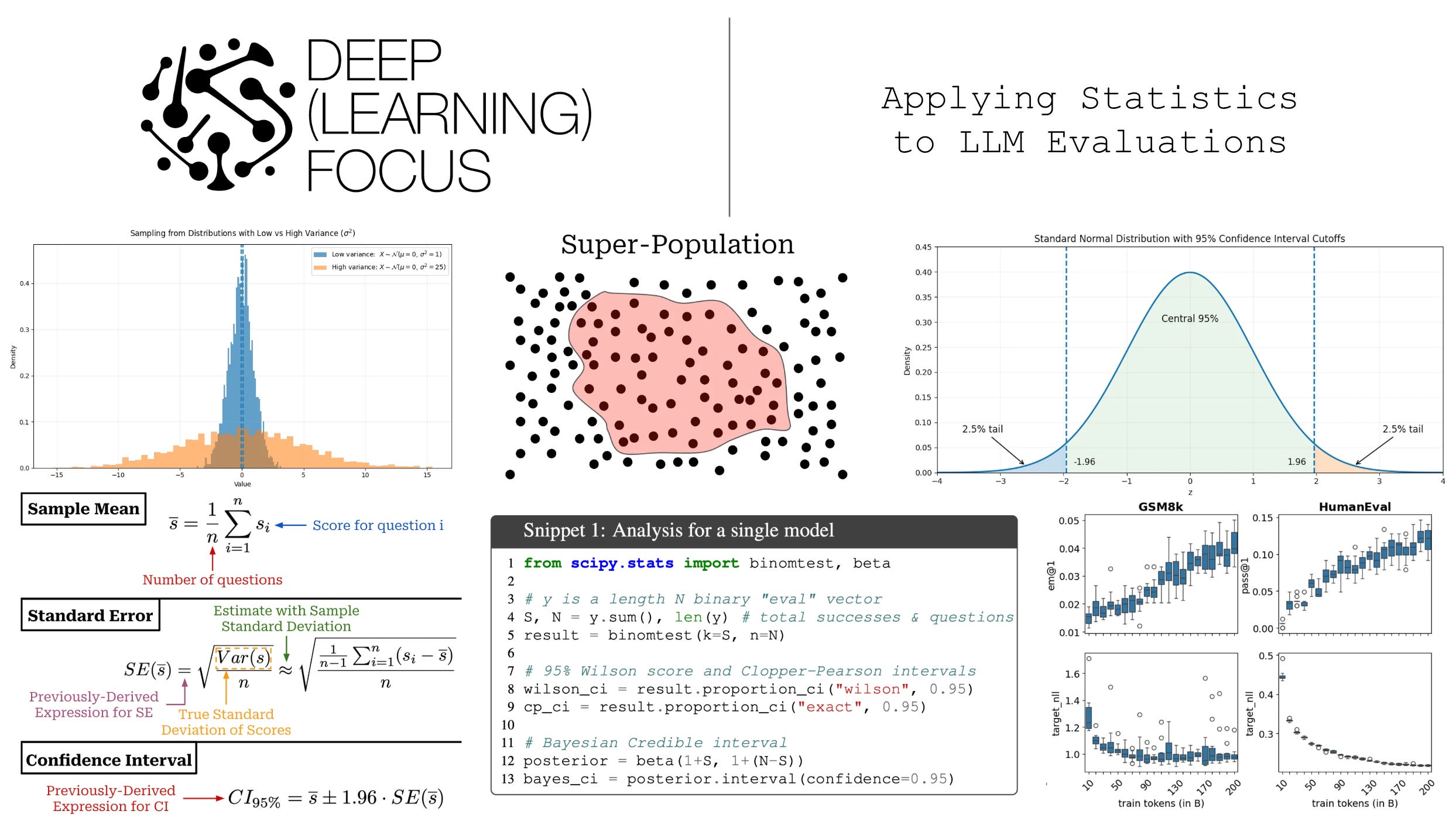
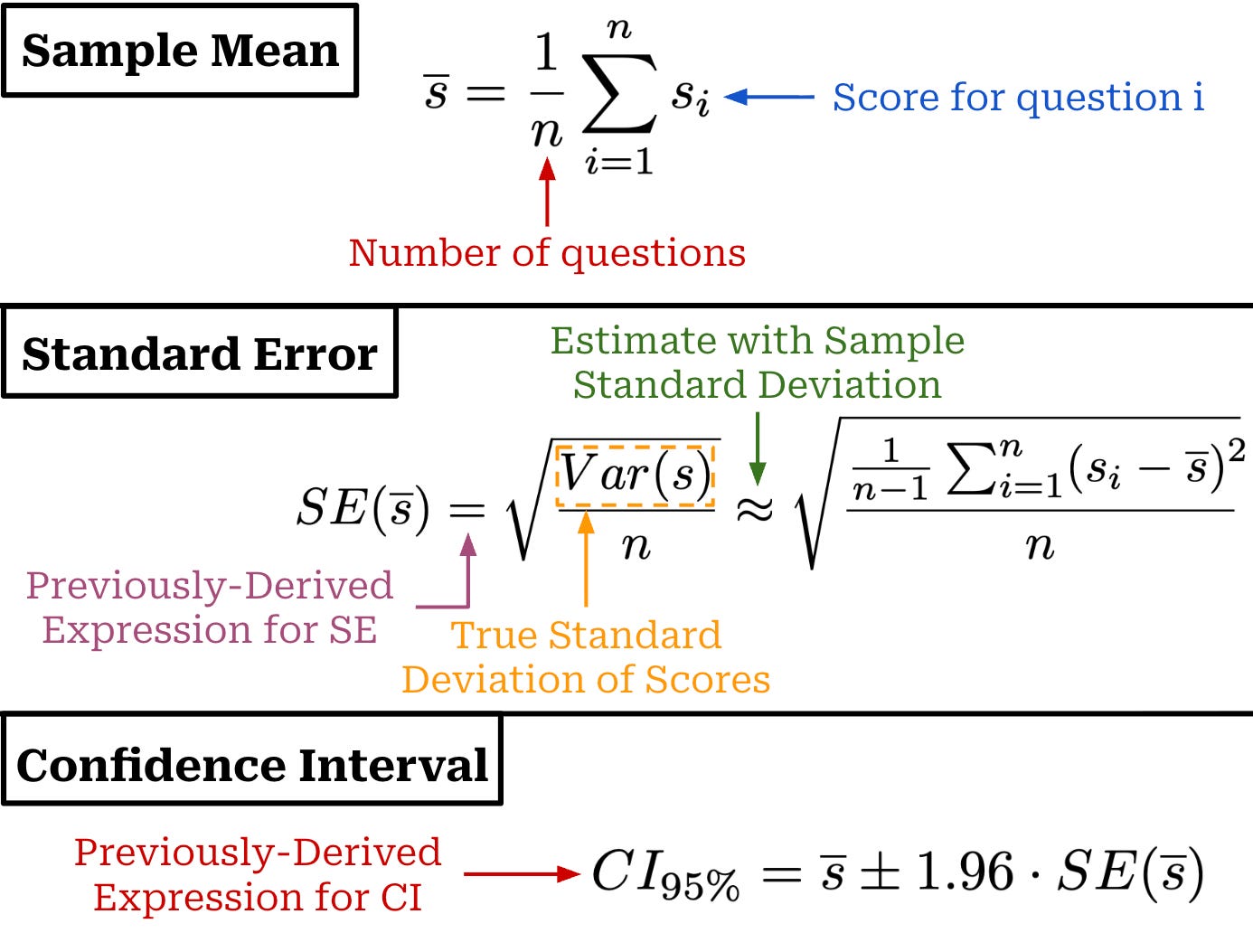
A random variable X is defined as a quantity that has a value dependent upon chance. We can take several independent samples from the distribution {x_1, x_2, …, x_n}, and the values of these observations will be sampled from the distribution of X (i.e., x_i ~ X). We define the mean (or average) of this random variable via the expectation, which can be computed in a continuous or discrete fashion as shown in the figure below. Additionally, we can compute a sample mean by averaging the values of n observations sampled from the distribution.
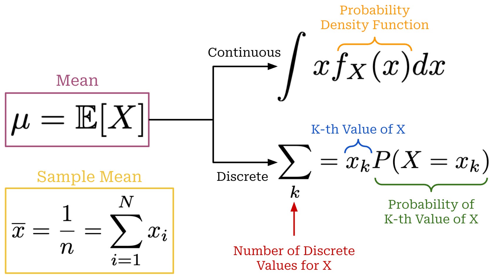
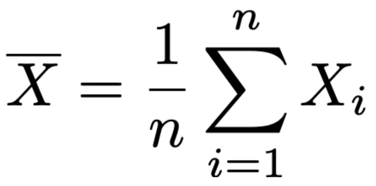
Formally, the lower case letters x_i represent concrete values sampled from a distribution, while upper case letter X_i denotes the i-th random variable in our sample—this is a notational detail, but it’s worth covering to avoid confusion. For example, if we evaluate our LLM on n questions, X_i is a random variable that represents the distribution of possible scores for question i1, while x_i is an actual evaluation score observed for a single evaluation run. We can also define the sample mean in terms of random variables as shown in the equation below. We use an uppercase X̄ in this case because we are defining a random variable.
The distribution of our random variable X also has variance Var(X), which describes how “spread out” the distribution is around the mean. In this overview, we will assume that this variance is finite (i.e., less than infinity). If we have a distribution with high variance, then samples taken from this distribution will be more spread out around the mean and vice versa; see below for an illustration.
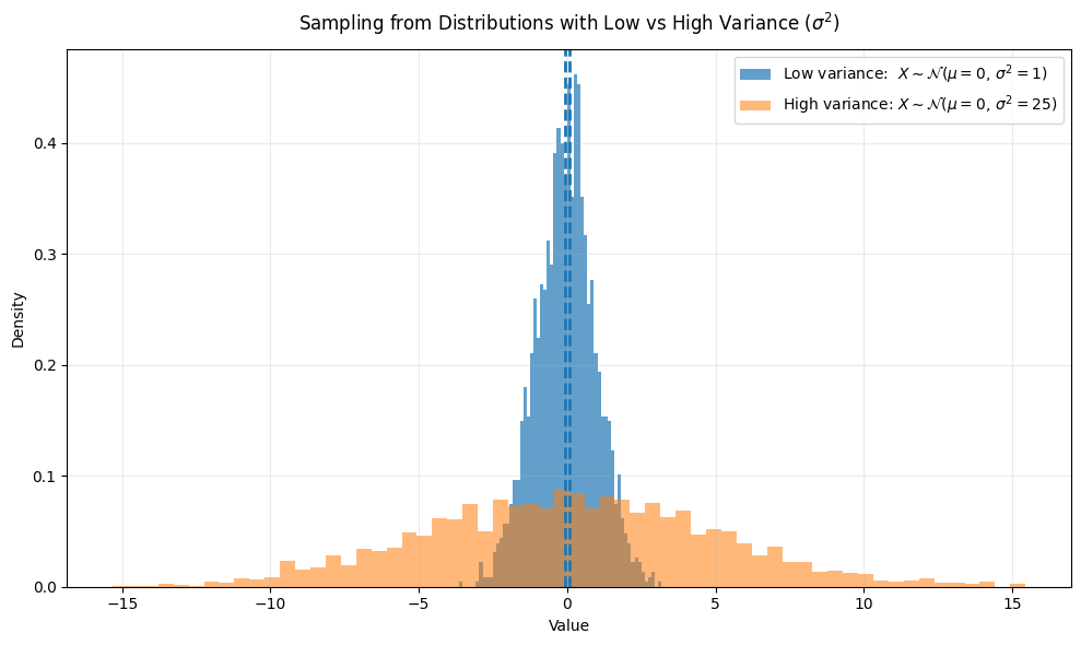
The expression for Var(X) is provided below. Similarly to the sample mean, we can also estimate variance using a fixed set of samples from our distribution X—this is how the variance is usually computed in practical settings. We can also compute the standard deviation σ by taking the square root of the variance. The variance and standard deviation describe the variability of individual samples from X.
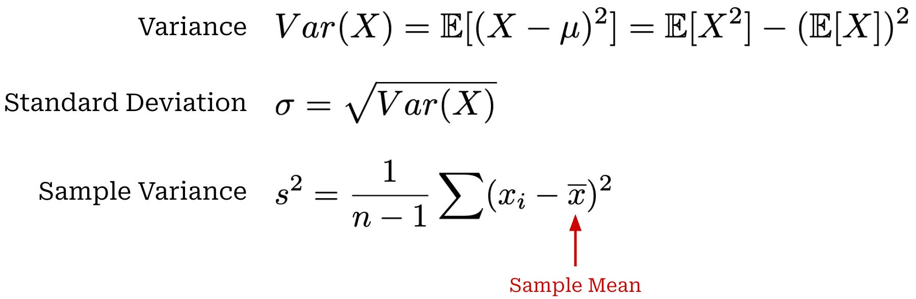
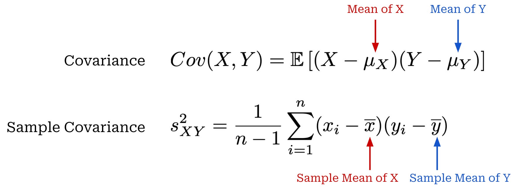
While variance measures the variability of a single random variable X, covariance measures how two random variables X and Y vary together. Intuitively, if these variables vary in the same direction (e.g., they are both above or below their means at the same time), then their covariance will be positive and vice versa. A covariance near zero indicates there is no clear relationship between X and Y. We can also compute a sample covariance similarly to the sample variance shown above. Expressions for covariance and sample covariance are provided below.
The law of total variance is a useful identity that decomposes the variance of a random variable X with respect to another random variable Y; see below. For the purposes of this overview, this law is useful because it lets us separate multiple sources of randomness in an evaluation result. Later, we will use it to decompose the variance of an evaluation score into two key components:
Variability due to the question sampled for evaluation.
Within-question variability arising from stochastic generation by the LLM or an LLM judge.

Standard Error and Sample Means
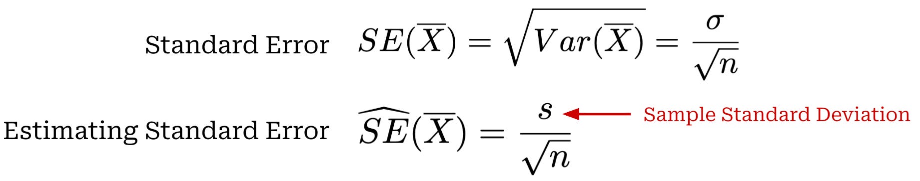
If we repeatedly draw samples from X and compute the sample mean, we will get a different result every time. The resulting sample means form a sampling distribution (i.e., basically a list of sample means we have drawn). The standard deviation of this sampling distribution is called the standard error of the sample mean. Put simply, the standard error is just the standard deviation over sample means. While the standard deviation captures variability in individual data points x_i sampled from X, the standard error captures variability in the sample mean estimator (i.e., the spread of sample means after computing it multiple times with different samples). A formal definition of the standard error is provided below, as well as an estimator for the standard error that uses sample standard deviation2 because the true value of σ is rarely known in practice and must be estimated.
This standard error equation makes the assumption that samples drawn from X are independent and identically distributed (IID). Independence implies that Cov(X_i,X_j) = 0 for i≠j, and identical distribution implies that each X_i has the same variance Var(X). From this assumption and a few other properties of the variance, we can derive the above expression for the standard error as shown below. The assumption of IID samples is not always satisfied—we should only use this expression when the samples being drawn are truly independent.
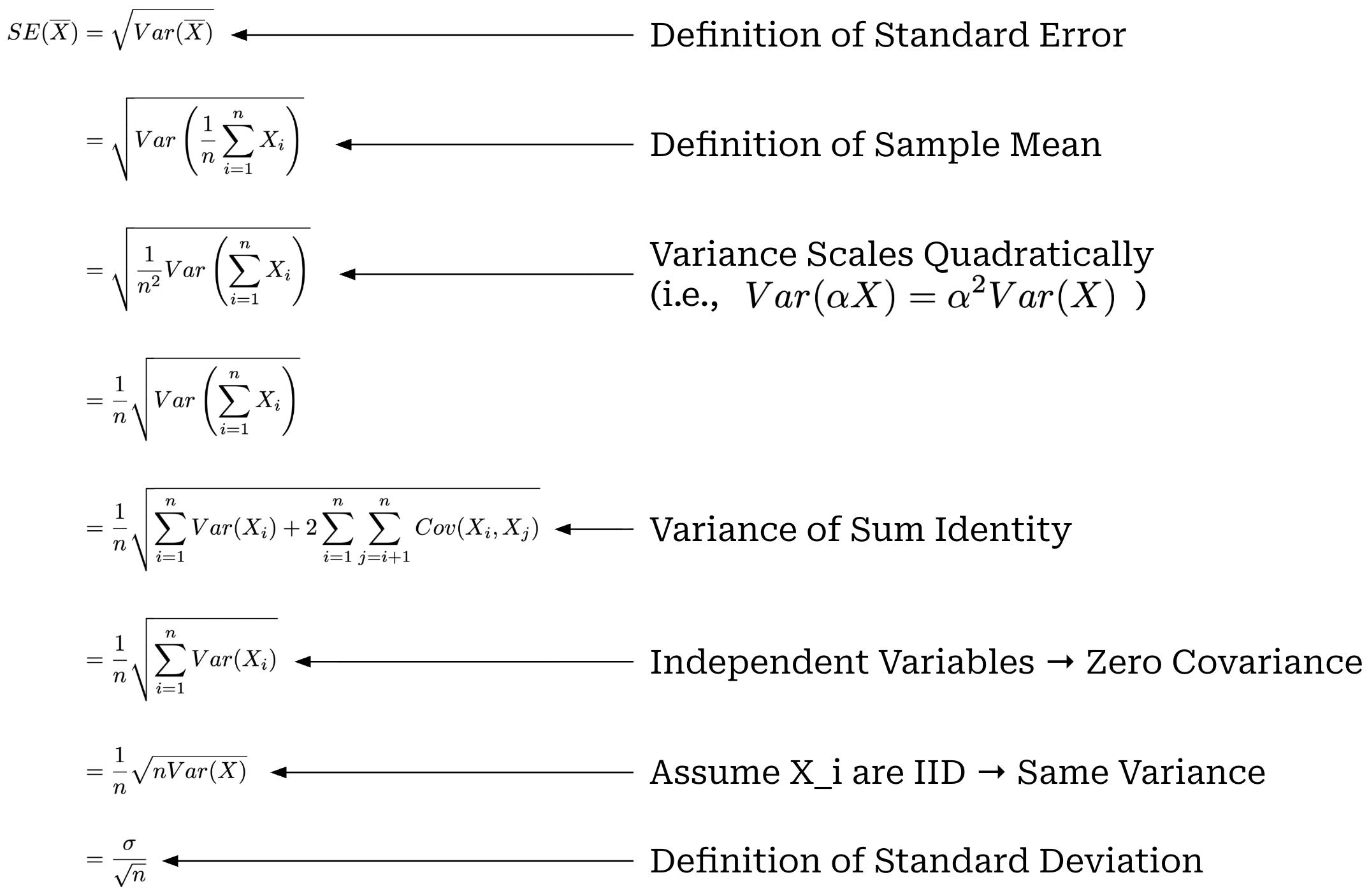
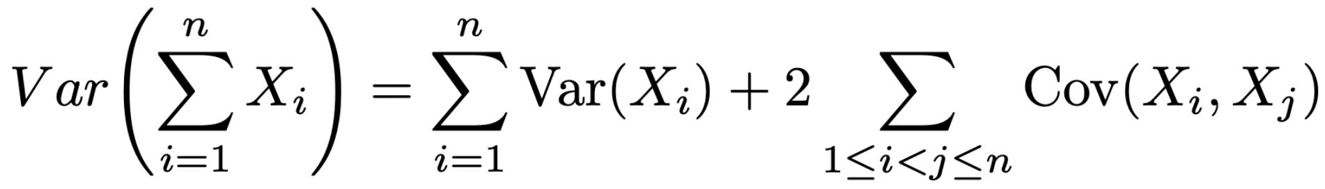
Within this derivation, we use the variance of a sum identity, which can be generally expressed as shown in the equation below. This identity allows us to capture the (non-zero) covariance terms within our variance expression.
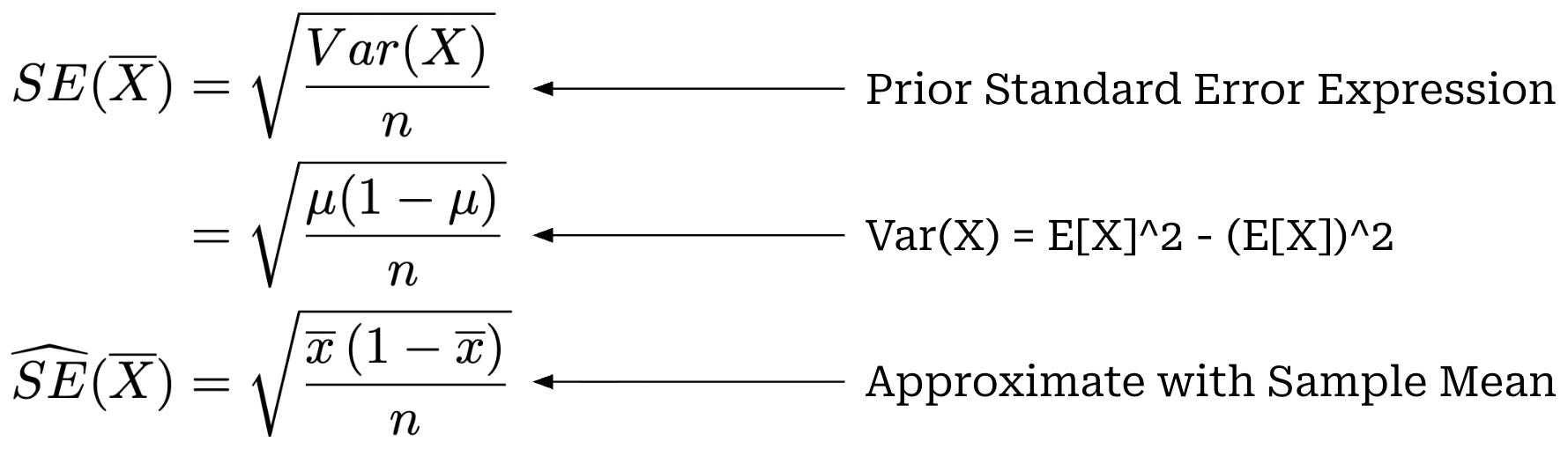
Bernoulli variables. Let’s assume X is a Bernoulli random variable, meaning that our scores are binary x_i ∈ {0, 1}. In this case, our standard error expression can be simplified even further. To begin, we know that E[X] = 1×P(X=1) + 0×P(X=0) = P(X=1). Given that the values of X are either zero or one, it is also true that E[X^2] = E[X] because x^2 = x when x = 0 or x = 1.
We can easily plug these two identities into our prior expression for the variance Var(X) = E[X^2] - (E[X])^2 = Pr(X=1) - (Pr(X=1))^2 = μ(1 - μ), where μ is the mean of X. Practically, we can estimate μ by taking a sample mean X̄. Then, we can plug this simplified Var(X) into our previous formula for the standard error, yielding the simplified expression shown below. Therefore, we can use this simpler standard error expression when the values of X are binary.
Law of Large Numbers and the Central Limit Theorem (CLT)
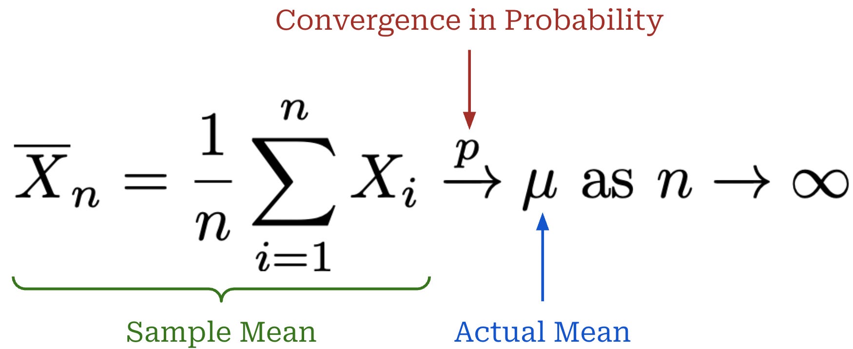
The law of large numbers is a fundamental concept in statistics that builds upon our prior definition of the sample mean. Given a random variable X, we are often interested in its true mean μ. This mean can be estimated with the sample mean over n samples, but this is a random estimate that can differ from μ. The law of large numbers tells us that as the value of n increases, the sample mean will approach (i.e., converge in probability) the true mean μ; see below.
The law of large numbers only tells us that the sample mean will eventually settle around μ with sufficiently large n. It does not tell us how much the sample mean differs from the true mean at finite n or how quickly we converge to μ as n increases. We can express the intuition for the law of large numbers as follows: with enough data, our estimator (i.e., the sample mean) approaches the true mean.
Standardization and z-score. Given a random variable X (or a realized value x), we can standardize by subtracting the mean μ and dividing by the standard deviation σ; see below. This process produces a standardized random variable Z (or a realized value z). The z-score z3 indicates how many standard deviations—in units of σ—the value x lies above (z > 0) or below (z < 0) the mean μ.
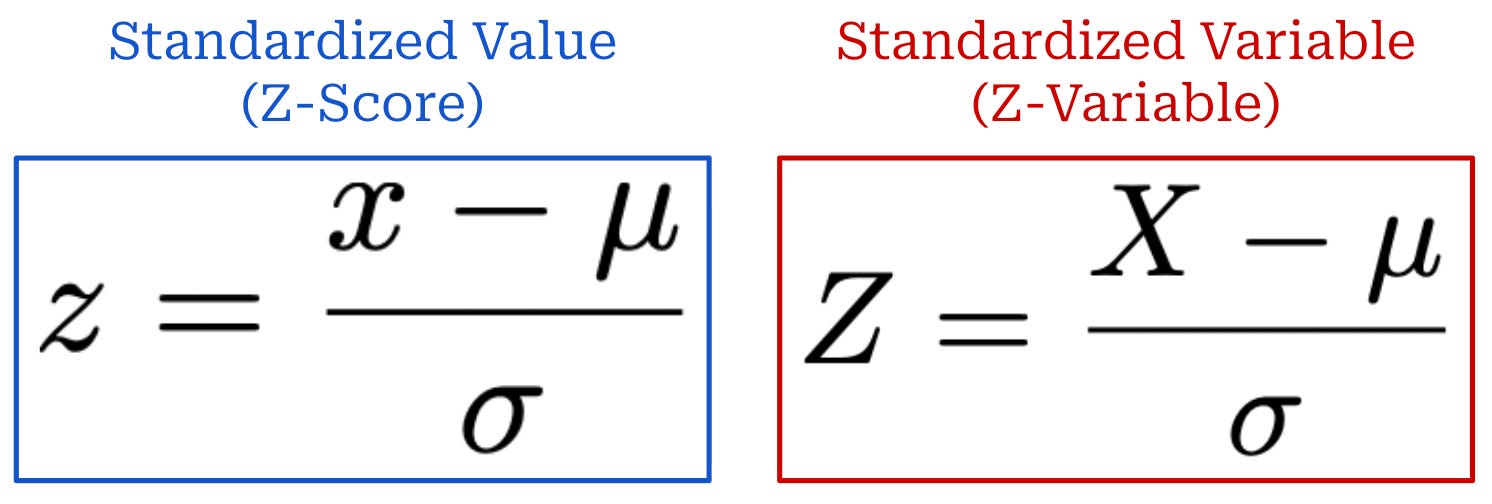
Any variable or value can be standardized in this way. For example, we will next standardize the sample mean while formulating the Central Limit Theorem.
The Central Limit Theorem (CLT) goes beyond the law of large numbers by describing how our sample mean estimates will be distributed around the true mean μ. Our random variable X has a mean of μ, and we estimate this mean with a sample mean. We know from our prior derivation that this sample mean has a variance of σ^2 / n (assuming IID random variables and finite variance σ^24).
Using this mean and variance, we can standardize the sample mean to obtain Z_n by subtracting the mean and dividing by the standard error; see below. The denominator of Z_n is our previous equation for standard error—this is just the standard deviation of our sample mean! We rarely know the actual value of σ, so we can estimate the true value with the sample standard deviation s.
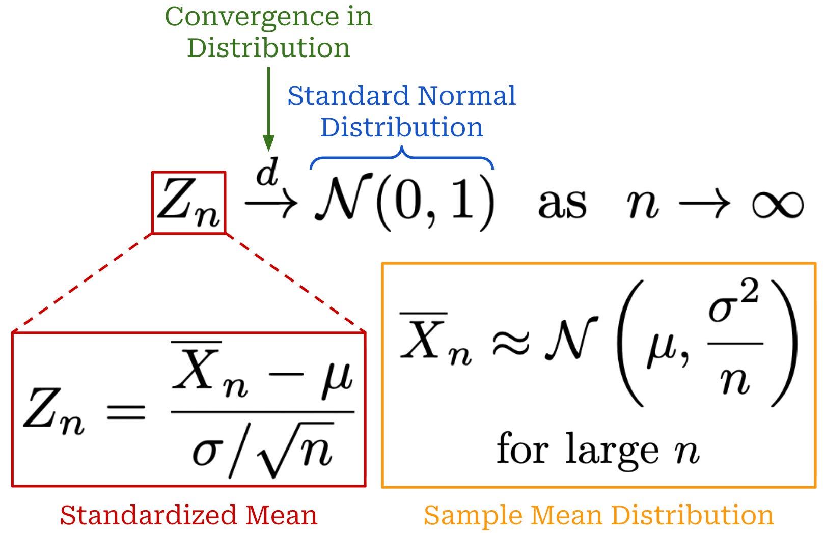
The CLT tells us that the distribution of Z_n will converge to a standard normal distribution5—meaning a normal distribution with a mean of zero and variance of one—as the value of n increases. Stated differently, this means that the distribution of our sample mean becomes approximately normal with sufficiently large n, as shown in the orange distribution above. From this information, we know that the standard deviation of the sample mean distribution will decrease proportionally to 1 / sqrt(n) and the error of our sample mean estimate is on the order of σ / sqrt(n)—the standard deviation of the above distribution.
Confidence Intervals
Consider a random variable X with a true mean μ that we estimate with the sample mean X̄_n computed from n samples. To quantify the uncertainty of this estimate, we can next compute a 95% confidence interval that has the following form: x̄_n ± y. This confidence interval indicates that if we repeated the sampling procedure many times and recomputed this confidence interval each time, 95% of the resulting confidence intervals would contain the true mean μ. Our goal is to find the value of y that statistically yields such a 95% confidence interval. To find a formula that allows us to compute this confidence interval, we actually need to combine all of the ideas we have learned so far.
First, let’s consider our sample mean estimator X̄_n. Assuming IID samples with finite variance, we know from the CLT that this estimator has an approximately normal distribution N(μ, σ^2 / n) assuming that the value of n is sufficiently large, as well as a standard error given by SE(X̄_n) = σ / sqrt(n). When computing a 95% confidence interval, we consider a normal distribution N(0, 1) and try to find a bound that includes 95% of the probability mass for this distribution; see below for an illustration.
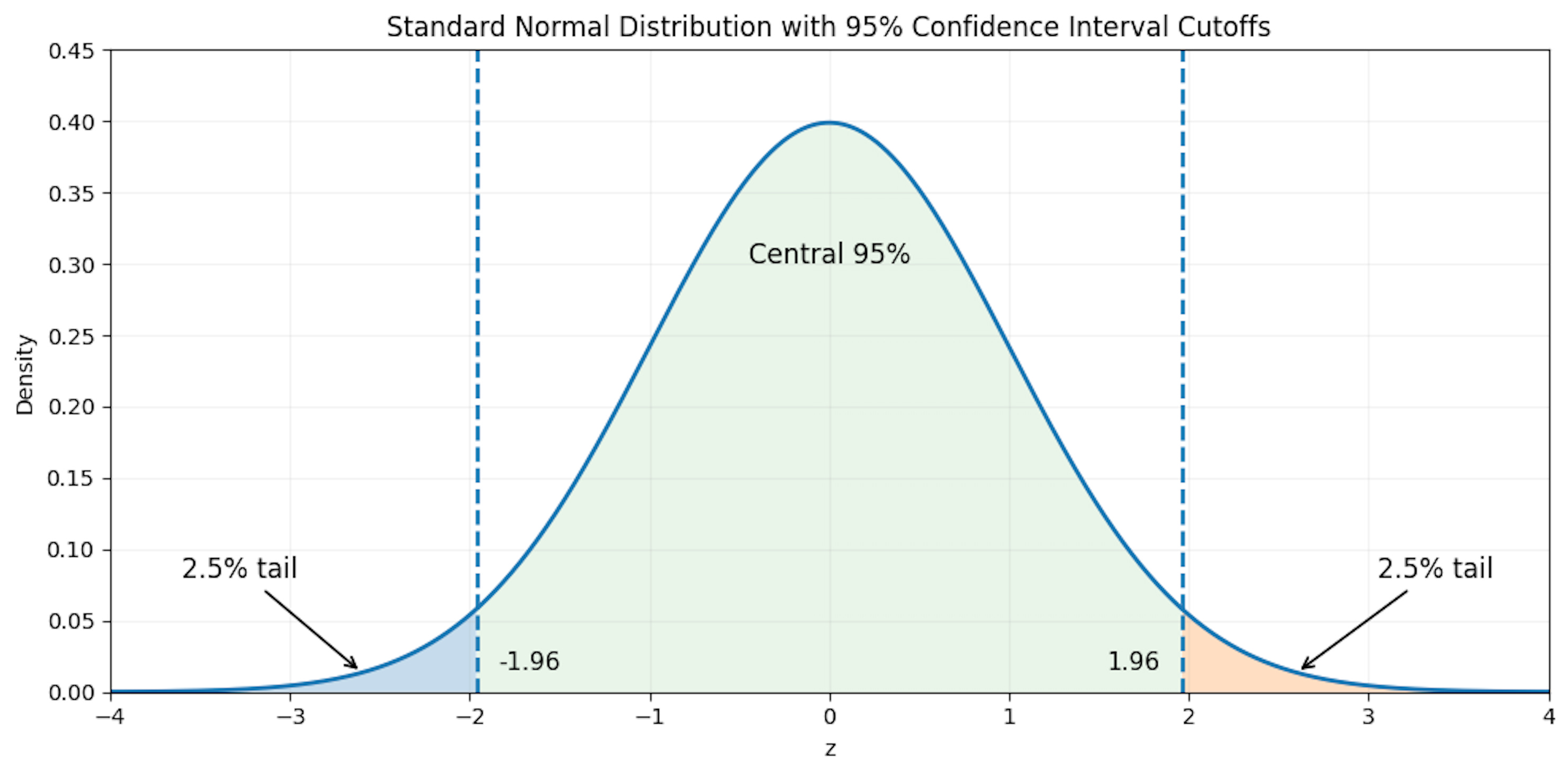
Given a standard normal distribution, we have P(|Z| < 1.96) = 0.95. This is a two-sided confidence interval, meaning 2.5% of the total 5% of probability mass outside our confidence interval is allocated to each side of the distribution. In most cases, however, we will want to compute a confidence interval for a non-standard normal distribution. To do this, we can just standardize the distribution as discussed previously. For example, given our distribution N(μ, σ^2 / n) from the CLT, we can derive a standardized variable Z that follows a standard normal distribution. From here, we can just transform the confidence interval with the same standardization process; see below.
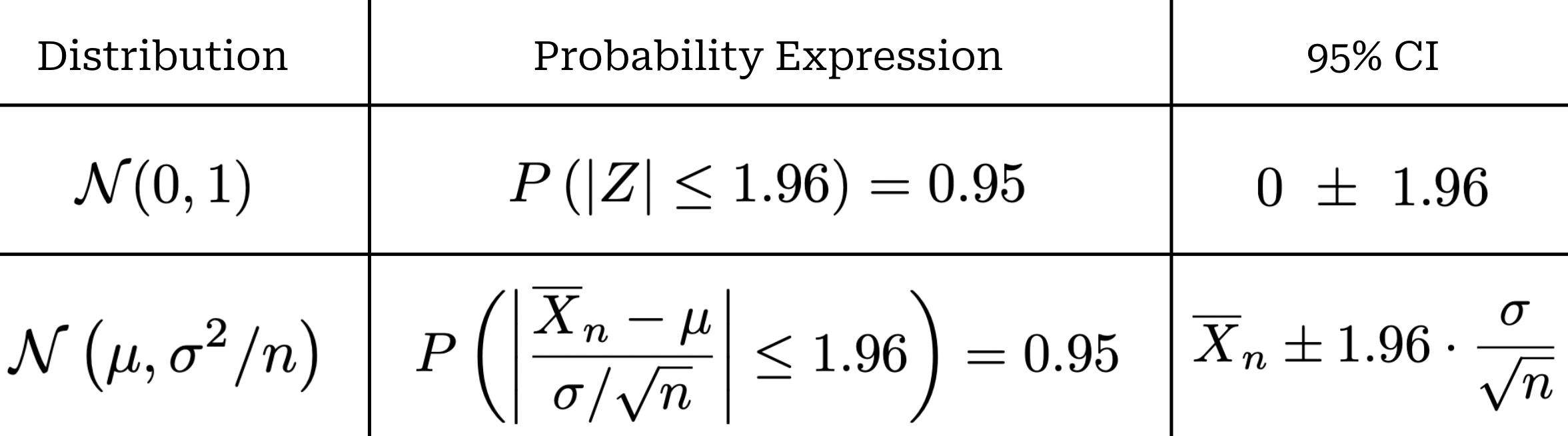
This approach yields a formula—based upon our sample size and the standard error of our sample mean—that can be used to compute a 95% confidence interval.
A Statistical Approach to LLM Evaluations [1]
Now that we have built a solid statistical foundation, we can use these ideas to create a framework for LLM evaluations that better quantifies uncertainty. In doing this, we can be more confident in our model evaluations and understand whether certain evaluation results are legitimate or just caused by noise. Our discussions will be based on a seminal paper from Anthropic [1] that provides several key recommendations for performing LLM evaluations in a way that is grounded in statistics, rather than just comparing raw performance metrics.
“Fundamentally, evaluations are experiments; but the literature on evaluations has largely ignored the literature from other sciences on experiment analysis and planning. This article shows researchers with some training in statistics how to think about and analyze data from language model evaluations.” - from [1]
Statistical framing for LLM evaluations. In theory, when evaluating an LLM, there exists a super-population of questions (illustrated below) that exhaustively covers all the ways in which the LLM can be evaluated. Practically speaking, any evaluation dataset represents only a finite subset of questions from this super-population, as represented by the red shaded region in the figure below.
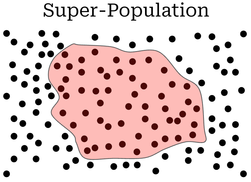
This framing can be used to rethink our perspective on model evaluations. Instead of trying to maximize the performance of our model on a finite benchmark, we should be trying to improve an underlying skill of the model. Any evaluation dataset captures a corresponding skill imperfectly, as it is only a finite sample from the super-population that is associated with that skill.
Key recommendations. There are a set of concrete recommendations proposed in [1] that outline how one can approach LLM evaluations in a rigorous manner. We first outline these recommendations here, then spend the rest of this section explaining each of them in more depth:
When questions are IID, LLM evaluation results should be accompanied by standard errors that are computed using the CLT.
If questions are not IID (e.g., drawn from related clusters or groups), then our CLT standard error formula is no longer valid and we should instead compute a clustered standard error.
To reduce the variance of evaluation results, we can re-sample outputs from the LLM multiple times—or even analyze next token probabilities—to better account for the variance of each individual evaluation result.
When comparing two models, we can perform analysis of their paired difference (i.e., rather than just providing separate, aggregated evaluation scores over the dataset) to yield a more confident result.
Preliminaries. The evaluation dataset in [1] is assumed to contain n questions, and each question receives an evaluation score s_i; e.g., a binary correctness signal or an LLM-as-a-Judge score. A score can be decomposed as s_i = x_i + ϵ_i, where x_i is the expected score (i.e., E[s_i] = x_i) and ϵ_i adds randomness to the score. We assume zero-mean randomness (i.e., E[ϵ_i|i] = 0) that does not change the expected score. Put simply, this setup models a non-deterministic evaluation setting. Notably, LLM evaluation is fundamentally non-deterministic, as it involves sampling from the next token distribution of one or more LLMs (i.e., the model being evaluated and possibly an LLM judge).
Standard Errors and the CLT
The simplest case when analyzing evaluation results is when each question i is independent. Our goal in analyzing an evaluation result is to understand the true performance of our model, represented by the mean score μ = E[s] = E[x]6 from our super-population. We only have access to a finite set of scores from our evaluation dataset. However, we know from the law of large numbers that we can estimate the true mean by taking a sample mean s̅ over a finite set of evaluation scores. This estimator approaches μ as the value of n becomes larger.
In other words, taking an average score over a large number of independently-sampled questions generally provides a good estimate of a model’s true performance. However, “good” is difficult to quantify, and how do we know if n is sufficiently large? To quantify uncertainty, we can use the CLT to compute the standard error for our sample mean; see above. As we can see, this expression is identical—other than switching x with s—to our previously-derived standard error expression. We can also derive a confidence interval from the standard error similarly to before.
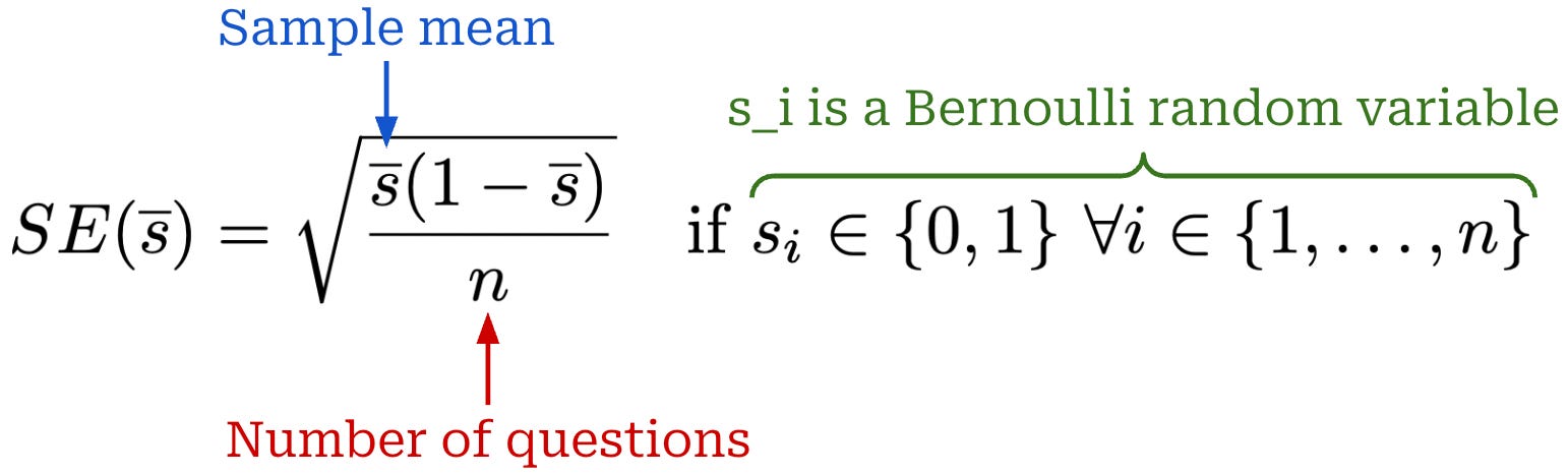
If we assume a Bernoulli distribution—meaning that for all i we have s_i ϵ {0, 1}—this expression can be simplified even further; see above. However, the Bernoulli formula requires that scores are truly binary (i.e., not fractional7).
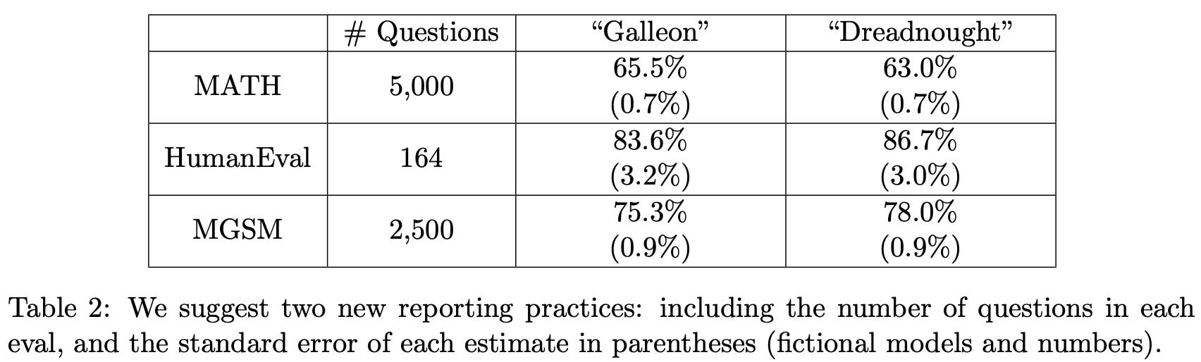
“We suggest reporting the standard error of the mean alongside (beneath) the mean when reporting eval scores.” - from [1]
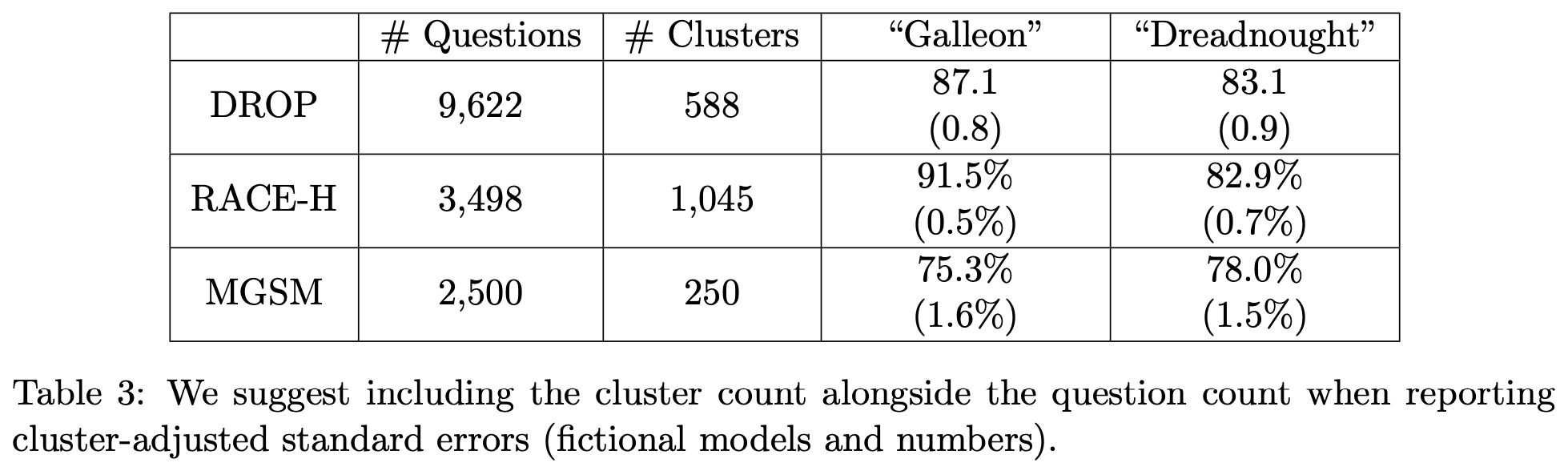
Now that we know how to compute these quantities for an LLM evaluation, the recommendation in [1] is simple: just report this standard error and the number of samples n alongside the actual evaluation result. Computing this standard error is not difficult—it requires forming a sample estimate of the standard deviation of s. A toy example of the proposed reporting structure for two models evaluated over three evaluation datasets is provided in the table below for reference.
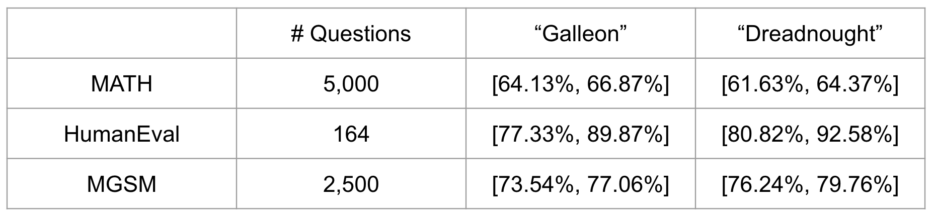
From the standard error, we can compute a confidence interval for each model’s evaluation metric. These intervals summarize uncertainty in the estimated mean performance. When comparing models, non-overlapping confidence intervals suggest a real performance difference, but overlapping intervals do not by themselves rule one out. A precise comparison requires directly analyzing the difference between the models, which we will handle in a future section.
As an example, confidence intervals for the table above have been computed below for all model and dataset combinations. We see here that all models have overlapping confidence intervals. In future sections, we will learn methods that can be used to compare models with a greater level of precision.
Bootstrapping is another common approach to use for evaluating machine learning models (including LLMs) that proceeds as follows:
Sample
nquestion scores with replacement.Compute the sample mean
s̅.Repeat steps 1-2 multiple times.
Measure the standard deviation of these sample means.
Use this standard deviation as an estimate of the standard error.
While this approach is valid and commonly used in LLM evaluations, authors in [1] argue that bootstrapping is unnecessary when the CLT is valid. Therefore, we can just use the CLT when questions are sampled independently, n is sufficiently large, and the variance of our scores is finite. However, the CLT does fall short when n is small—the handling of this evaluation regime is discussed extensively in [2].
Clustered Errors
“We show how to use clustered standard errors, a technique developed in the social sciences, to account for the dependence and correlation structure present in question clusters.” - from [1]
If questions are not sampled independently, the standard error expression from the CLT is no longer valid. In this case, the CLT underestimates uncertainty—our confidence intervals are too narrow. We are evaluating on n questions, but some of the questions are actually related to each other. As a result, the “effective” number of evaluation questions is smaller than n, thus increasing the standard error. Some practical examples of non-independent questions include:
The same prompt in different languages.
Prompts that reference the same document or source.
Questions that are generally related in format or topic.
To avoid underestimating uncertainty, authors in [1] recommend using a clustered standard error. We use s_{i, c} to denote the score for question i in cluster c. The cluster-adjusted standard error assumes that clusters are independent: questions in a cluster can be correlated, but questions across clusters cannot.
To evaluate an LLM on these clusters, we still compute the sample mean across all question scores S̅, but we modify our standard error expression. Before, we assumed that scores S_i were IID, which implies that Cov(S_i, S_j) = 0 when i ≠ j. When questions are clustered, we no longer have zero covariance, so we need to adjust our derivation of the standard error; see below.
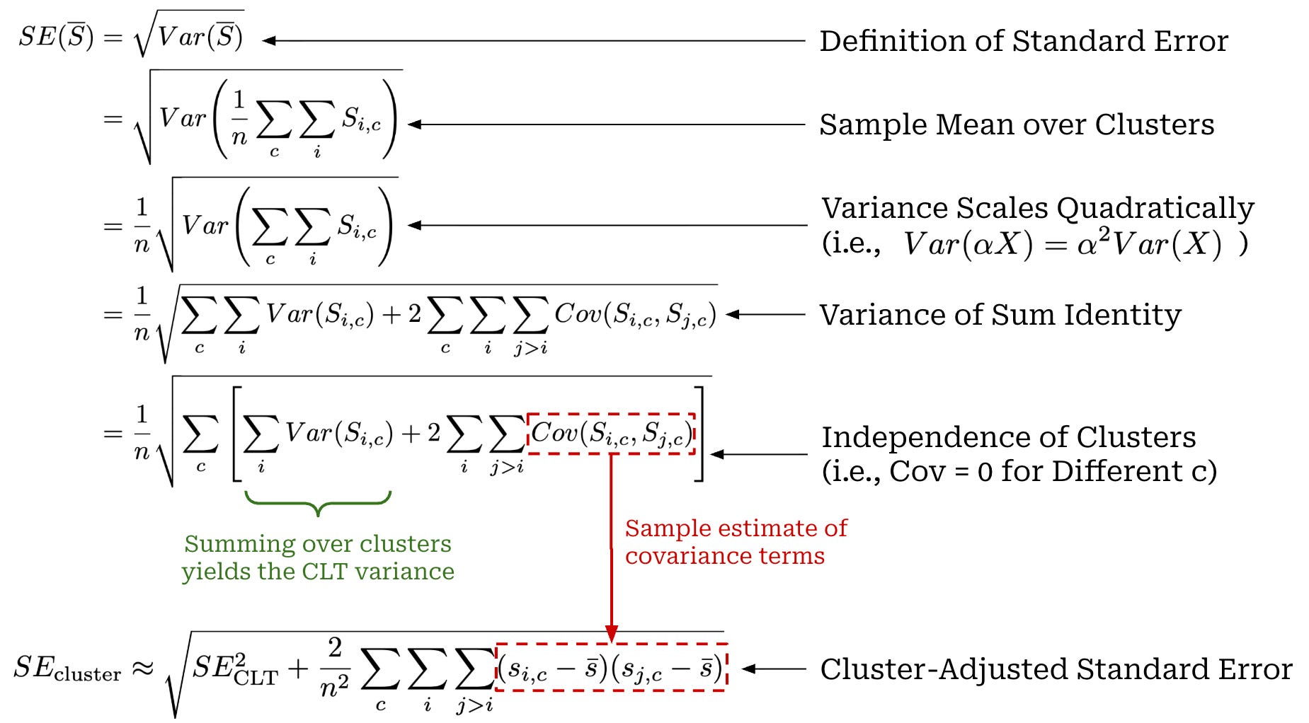
The above clustered standard error equation interpolates between two cases:
Scores within a cluster are perfectly correlated and each cluster is treated as if it were a single question
i.Scores within a cluster have no correlation, so our expression reduces to the original standard error expression from the CLT.
“The clustered standard error acts as a kind of sliding scale between cases where scores within a cluster are perfectly correlated (in which case each cluster acts as a single independent observation) and perfectly uncorrelated (in which case the clustered standard error is equivalent to the unclustered case). The intra-cluster correlations… are captured by the triple summation (over clusters and cross-terms within clusters).” - from [1]
When questions are not sampled independently, authors in [1] recommend reporting cluster-adjusted standard errors, as well as the number of questions n and the number of clusters C; see below. Similarly to before, the cluster-adjusted standard error can be used to compute a confidence interval. In practice, the clustered standard error may be drastically larger than the CLT standard error. For example, authors provide a concrete example in [1] where the standard error increases by 3× when accounting for clusters. Failing to consider whether questions are actually independent can drastically impact the interpretation of evaluation results.
We assume that questions are sampled independently in future sections unless stated otherwise. However, we can use similar steps as outlined above to derive most results in a cluster-adjusted fashion. Many of the derivations extend to the clustered setting once the covariance structure is accounted for appropriately.
Reducing Variance
We now understand how to compute standard errors and confidence intervals for our evaluation results. The next reasonable question to ask is: What can we do to reduce the standard error? First, recall that our evaluation score is defined as s_i = x_i + ϵ_i, where we have E[s_i] = x_i and Var(ϵ_i) = σ_i^2. To answer this question, we begin with our expression for the standard error and perform a decomposition with the law of total variance; see below.
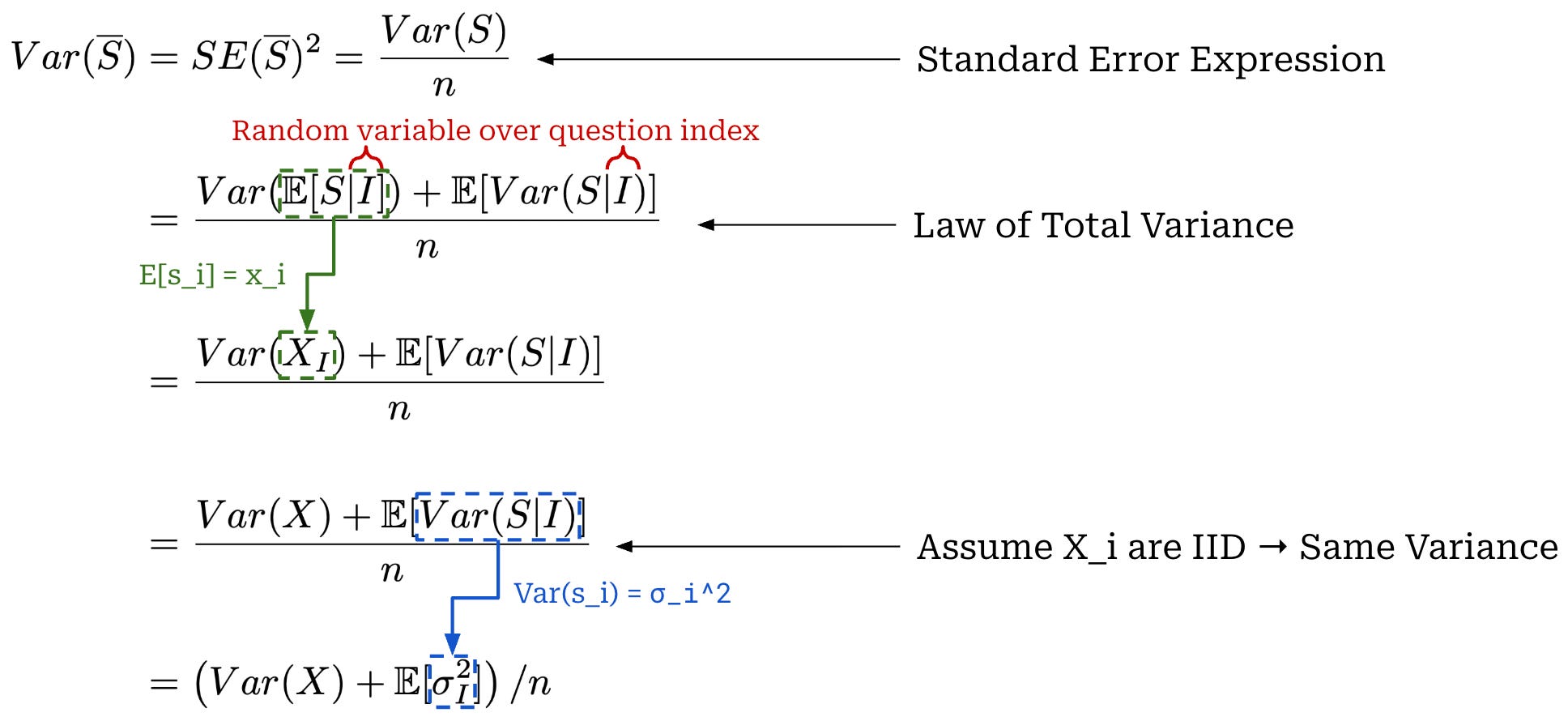
To apply the law of total variance, we use the following two random variables:
A random variable over evaluation scores
S.A random variable over the question that gets sampled
I.
We apply the law of total variance by conditioning S on I, where X_I = E[S|I] is the expected score for the sampled question I. We can then further simplify the equation using known properties of the mean and variance of a score.
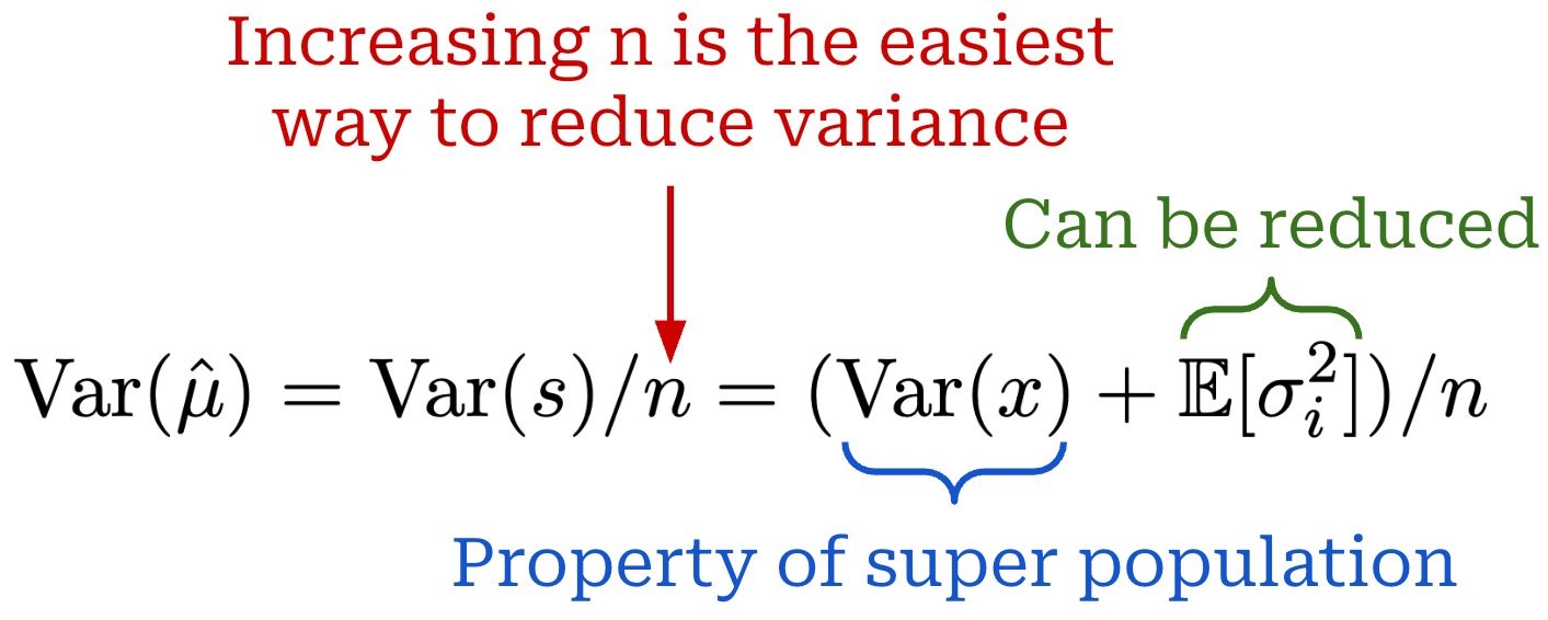
This derivation yields the variance expression shown above, which provides some actionable insights. First, we see that the simplest method for reducing variance is simply increasing n—evaluating over a larger set of questions naturally improves reliability. Additionally, Var(x) captures the variability in the mean score across our evaluation dataset—this is a fundamental property of our super-population that cannot be easily changed. In simple terms, this quantity captures the spread in question difficulty across all possible evaluation questions. However, there are several approaches we can explore for decreasing the value of E[σ_i^2].
Resampling can be used to reduce score variance when evaluating any model. Instead of generating and scoring a single output per question, we generate and score K outputs for the same question i (i.e., by sampling multiple completions from the LLM). In [1], authors assume that resampled scores for a fixed question i are IID. After sampling K scores, we can take an average of the scores S̅_i, which decreases the score variance by a factor of K; see below for a full derivation.
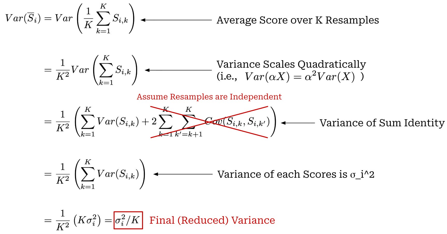
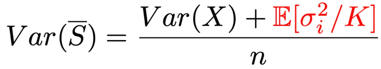
Therefore, resampling—or producing K scores for question i to yield a mean score S̅_i—provides a linear reduction of the within-question variance σ_i^2 compared to using a single score. The variance for our sample mean has two key terms—Var(x) and E[σ_i^2]—that are summed together in the numerator. As mentioned before, Var(x) is not mutable, so to reduce variance we can—in addition to increasing n—increase the value of K until E[σ_i^2 / K] ≪ Var(X). By doing this, the within-question variance term shrinks toward zero and the variance of our sample mean approaches Var(x) / n; see below.
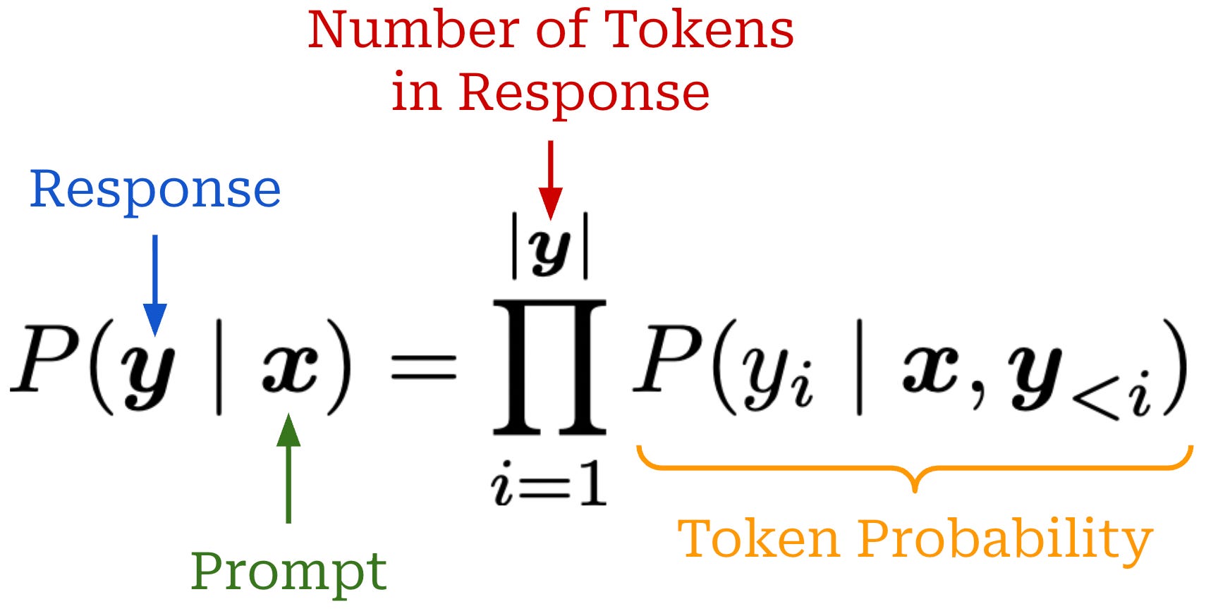
Token probabilities. If an evaluation metric can be computed from the model’s next token probabilities, we can replace a sampled score with its conditional expectation—basically just the probability of the correct response—and remove the within-question variance (i.e., meaning that σ_i^2 = 0). Using output token probabilities, we can easily compute the probability of a response from our LLM. For example, if our response is just a single token (e.g., a multiple choice answer), then we know that the probability for this score is the probability of that token within the LLM’s next token distribution. If our response is more complex (i.e., multiple tokens), then we can also compute the probability of the entire response via the product of probabilities for each individual token; see below.
For a question i, we will refer to the probability of a response to this question as p_i. If we have access to this probability, then we can use s_i = x_i = p_i, and the variance term for our score goes away (i.e., σ_i^2 = 0). As a result, directly using token probabilities is an effective variance reduction technique. In [1], authors also recommend against changing the sampling temperature—both for resampling and with token probabilities—because this alters the underlying response distribution and, in turn, the evaluation target. For this reason, these results study a different model configuration that is not fully comparable to our original LLM.
“We recommend a two-pronged variance-reduction strategy. When next-token probabilities are available, and the LLM eval can be conducted using next-token probabilities (i.e. without token generation), compute the expected score for each question, and compute the standard error of expected scores across questions. When next-token probabilities are not available, or the answer requires a chain of thought or other complex interaction, choose a K such that E[σ_i^2] / K ≪ Var(x) and compute the standard error across question-level mean scores. In neither case should the sampling temperature be adjusted for the sake of reducing variance in the scores.” - from [1]
Going further, we should note that this approach cannot be used in all cases. First of all, many closed LLMs do not provide direct access to token probabilities. Even if these probabilities are available, using them to compute p_i can be complex depending on the evaluation setup. For example, long-form responses with many tokens—though their probability can be computed—will usually be evaluated with an LLM judge, which uses a sampling procedure of its own and, therefore, adds variability into the resulting score. Additionally, recent reasoning models output a reasoning trajectory alongside their final response, which makes computing the output probability more complicated. In these cases, correctly computing p_i is not straightforward, and we cannot assume zero variance by setting x_i = p_i. In these cases, the resampling strategy described above is a better approach.
Model Comparisons
Now that we deeply understand how to analyze an evaluation score for a single model, we need to focus more on properly comparing the evaluation results of multiple different models. Usually, the goal of evaluation is to understand the performance of a model with respect to other models; e.g., determining if a new model version is better than the current or creating a leaderboard of the best models for a certain evaluation task. Although the techniques we have learned about so far can be applied to comparing evaluation results, we can usually make comparisons more statistically efficient by performing a pairwise analysis.
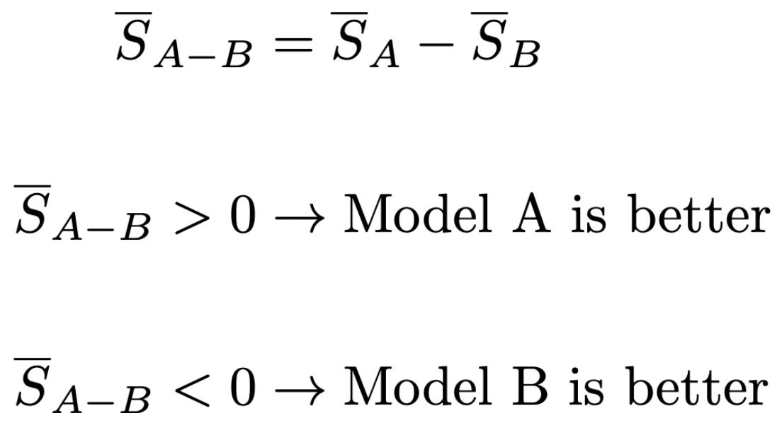
Difference of means. As we saw when learning about standard errors and confidence intervals, a common comparison heuristic is to compute separate confidence intervals for multiple models and check whether they overlap. If two 95% confidence intervals do not overlap, then there is a statistically significant difference between the evaluation results. As we will see, however, this test is actually overly conservative for detecting performance differences—intervals can overlap even when there is a statistically significant difference in mean scores. Instead, we can analyze the difference in mean between two models; see below. We will refer to the two models being compared as model A and model B for simplicity.
We can compute the standard error of the estimated difference in mean scores; see below. The standard error of the estimated difference in means is the square root of the sum of the variances of the mean estimators for models A and B.
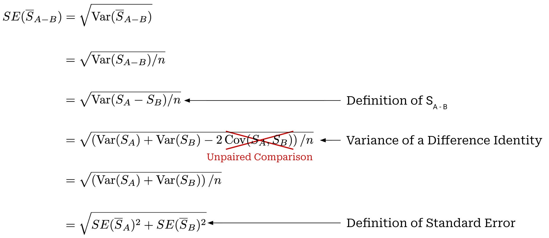
In this derivation, we use the variance of a difference identity, as expressed below. This identity is a special case of the variance of a sum identity we saw previously. In [1], authors consider an unpaired comparison where S̅_A and S̅_B are treated as estimates from independent evaluation runs (e.g., computed on independent question samples) such that Cov(S_A, S_B) = 0. This unpaired assumption could be violated (e.g., if models are evaluated over the same set of questions)—we should use the paired analysis from the next section in this case.

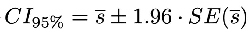
We can easily compute a 95% confidence interval using this standard error. To determine if one model is better than the other, we can check whether this confidence interval overlaps with a value of zero. If the 95% confidence interval does not include zero, then—assuming the true difference is zero—there is less than a 5% chance that we would observe a difference this extreme. Our expression for computing a 95% confidence interval has been copied below for convenience.
For model A to outperform model B according to this confidence interval, the difference in the mean score of models A and B must be greater than 1.96 × sqrt(SE_A^2 + SE_B^2). If we compute separate confidence intervals for each model, then this same difference must be greater than 1.96 × (SE_A + SE_B), which is stricter. In this way, checking overlap of separate confidence intervals is conservative, while constructing a confidence interval using the difference—and checking whether it excludes zero—is a better test.
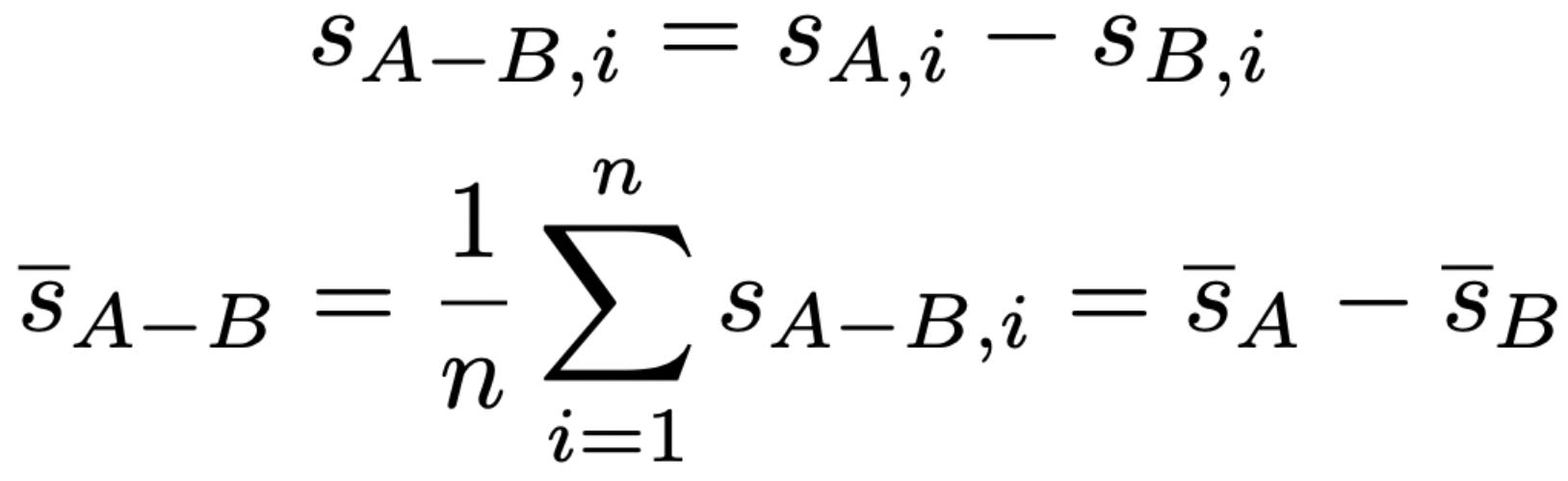
Paired difference. If models A and B evaluate on the same set of questions, we can further reduce variance by analyzing the question-level differences in scores. To begin, we can define question-level paired score differences as shown below.
We can then estimate the standard error of question-level score differences by drawing upon our same standard error expression used previously; see below. We can then use this standard error to compute confidence intervals like before.
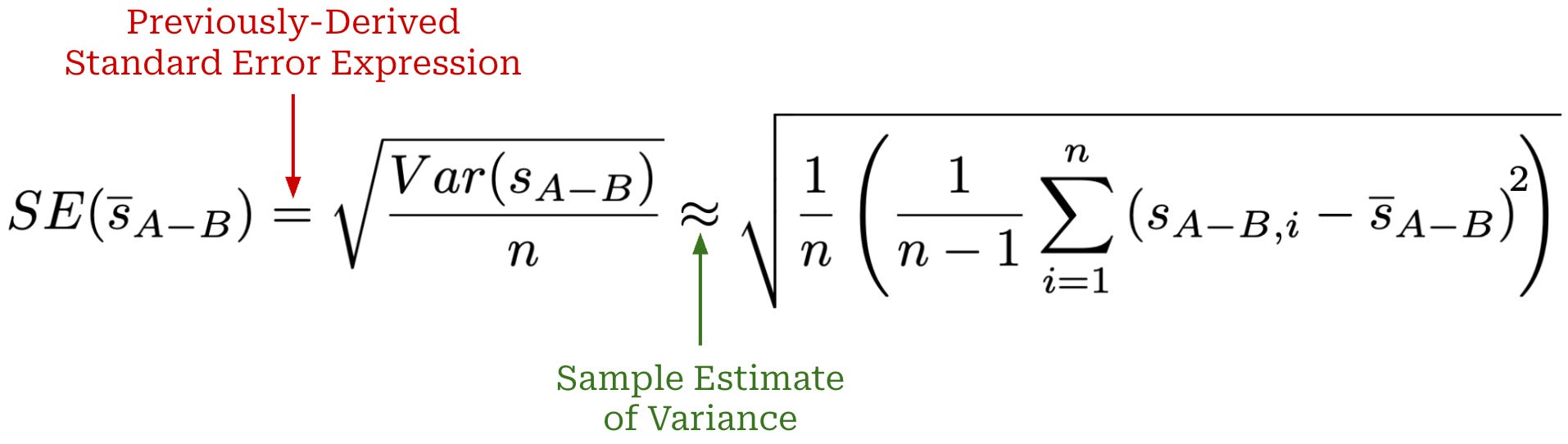
We can compute this standard error as shown above, but we are mostly interested in understanding whether this expression provides a meaningful reduction in variance. Ideally, we want the above paired standard error to be smaller than that of the difference of means so that we can better detect statistically significant model differences. To determine if this is the case, we can expand the above variance expression using the variance of a difference identity; see below. Unlike the prior unpaired analysis, we no longer assume that this covariance is zero.

The variance reduction for the above expression depends upon whether the mean scores of models A and B are correlated or not. If so, then this covariance term will be positive and we will see a corresponding reduction in variance. Intuitively stated, a positive correlation indicates that models A and B agree on whether certain prompts are easy or hard (i.e., per-item scores are directionally similar).
“Because eval question scores are likely to be positively correlated, even across unrelated models, paired differences represent a “free” reduction in estimator variance when comparing two models. We therefore recommend using the paired version of the standard error estimate wherever practicable.” - from [1]
In practice, most LLMs tend to agree on per-prompt difficulty, so analyzing paired differences is a useful approach that can offer meaningful reductions in variance. In [1], authors recommend reporting pairwise differences, standard errors, confidence intervals, and score correlations between models; see below.
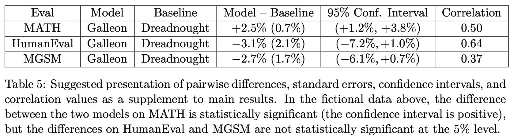
Practical Implementation
Although we have learned a lot of statistics throughout this discussion, actually implementing these ideas—once we understand them—does not add much extra complexity to the evaluation process. Computing standard errors and confidence intervals is straightforward and, once an implementation is available, can be readily adopted as a standard practice for model evaluations. However, we must be wary of the key assumptions being made when computing the standard error to avoid overconfidence; e.g., questions that are not independent require a cluster-adjusted standard error. A reference implementation of the techniques we have learned so far is provided below. This implementation outlines how all of the recommendations proposed in [1] can be applied when evaluating an LLM.
import math
import numpy as np


#################################
# Evaluation settings and scores
#################################

# model names
model_a_name = "Galleon"
model_b_name = "Dreadnought"

# example scores for the models (n = 10)
model_a = np.array([1, 1, 0, 1, 0, 1, 1, 0, 1, 1], dtype=float)
model_b = np.array([1, 0, 0, 1, 0, 1, 0, 0, 1, 1], dtype=float)

# form toy clusters
# two clusters, assignment based on even / odd index
clusters = np.array([i % 2 for i in range(len(model_a))])

# z score for 95% confidence interval
Z_95 = 1.96


####################
# Utility functions
####################

def mean_score(scores):
    return float(np.mean(scores))

def sample_sd(scores):
    return float(np.std(scores, ddof=1))

def ci_95(mean, se):
    return (mean - Z_95 * se, mean + Z_95 * se)

def fmt_pct(x):
    return f"{100 * x:.1f}%"

def fmt_pct_paren(x):
    return f"({100 * x:.2f}%)"

def fmt_ci(ci):
    return f"({100 * ci[0]:.2f}%, {100 * ci[1]:.2f}%)"


########################################################
# CLT SE
#
# Standard CLT SE for the sample mean: SE = s / sqrt(n)
# where s is the sample standard deviation.
########################################################

def clt_standard_error(scores):
    n = len(scores)
    return sample_sd(scores) / math.sqrt(n)


#####################################################
# Clustered SE
#
# Cluster-adjusted standard error:
# \sqrt{
#     SE_{CLT}^{2}
#     +
#     \frac{1}{n^{2}}
#     \sum_{c}\sum_{i}\sum_{j\neq i}
#     (s_{i,c} - \overline{s})(s_{j,c}-\overline{s})
# }
#####################################################

def clustered_standard_error(scores, clusters):
    n = len(scores)
    s_bar = np.mean(scores)

    # clt variance
    se_clt_sq = clt_standard_error(scores) ** 2

    # within-cluster cross terms
    cross_terms = 0.0
    for c in np.unique(clusters):
        idx = (clusters == c)
        residuals = scores[idx] - s_bar
        cross_terms += residuals.sum()**2 - np.sum(residuals**2)

    var_hat = se_clt_sq + (cross_terms / (n**2))
    return math.sqrt(var_hat)


######################################
# Summary statistics for single model
######################################

def summarize_model(scores, clusters):
    mean = mean_score(scores)

    se_clt = clt_standard_error(scores)
    ci_clt = ci_95(mean, se_clt)

    se_cluster = clustered_standard_error(scores, clusters)
    ci_cluster = ci_95(mean, se_cluster)

    return {
        "mean": mean,
        "se_clt": se_clt,
        "ci_clt": ci_clt,
        "se_cluster": se_cluster,
        "ci_cluster": ci_cluster,
        "n": len(scores),
        "num_clusters": len(np.unique(clusters)),
    }


###########################################################
# Comparing models w/ difference in means and separate SEs
###########################################################

def difference_in_means(scores_a, scores_b, clusters_a=None, clusters_b=None):
    mean_a = mean_score(scores_a)
    mean_b = mean_score(scores_b)
    diff = mean_a - mean_b

    # CLT version
    se_a_clt = clt_standard_error(scores_a)
    se_b_clt = clt_standard_error(scores_b)
    se_diff_clt = math.sqrt(se_a_clt ** 2 + se_b_clt ** 2)
    ci_diff_clt = ci_95(diff, se_diff_clt)

    # Clustered version
    if clusters_a is not None and clusters_b is not None:
        se_a_cluster = clustered_standard_error(scores_a, clusters_a)
        se_b_cluster = clustered_standard_error(scores_b, clusters_b)
        se_diff_cluster = math.sqrt(se_a_cluster ** 2 + se_b_cluster ** 2)
        ci_diff_cluster = ci_95(diff, se_diff_cluster)
    else:
        se_diff_cluster = None
        ci_diff_cluster = None

    return {
        "diff": diff,
        "se_diff_clt": se_diff_clt,
        "ci_diff_clt": ci_diff_clt,
        "se_diff_cluster": se_diff_cluster,
        "ci_diff_cluster": ci_diff_cluster,
    }


##########################################################
# Comparing models with paired instance-level differences
##########################################################

def paired_differences(scores_a, scores_b, clusters=None):
    diffs = scores_a - scores_b
    mean_diff = mean_score(diffs)

    se_paired_clt = clt_standard_error(diffs)
    ci_paired_clt = ci_95(mean_diff, se_paired_clt)

    if clusters is not None:
        se_paired_cluster = clustered_standard_error(diffs, clusters)
        ci_paired_cluster = ci_95(mean_diff, se_paired_cluster)
    else:
        se_paired_cluster = None
        ci_paired_cluster = None

    # Correlation between model scores across questions
    corr = float(np.corrcoef(scores_a, scores_b)[0, 1])

    return {
        "diffs": diffs,
        "mean_diff": mean_diff,
        "se_paired_clt": se_paired_clt,
        "ci_paired_clt": ci_paired_clt,
        "se_paired_cluster": se_paired_cluster,
        "ci_paired_cluster": ci_paired_cluster,
        "correlation": corr,
    }


############################################
# Functions to recreate tables from paper
#
# Numbers will not match exactly because we
# hard-code model scores at top of script
############################################

def print_table_2_style(model_name, summary):
    print(f"| {model_name:12s} | "
          f"mean = {fmt_pct(summary['mean']):>6s}  "
          f"SE = {fmt_pct_paren(summary['se_clt']):>8s}  "
          f"95% CI = {fmt_ci(summary['ci_clt'])}  "
          f"n = {summary['n']}")

def print_table_3_style(model_name, summary):
    print(f"| {model_name:12s} | "
          f"mean = {fmt_pct(summary['mean']):>6s}  "
          f"clustered SE = {fmt_pct_paren(summary['se_cluster']):>8s}  "
          f"95% CI = {fmt_ci(summary['ci_cluster'])}  "
          f"n = {summary['n']}, clusters = {summary['num_clusters']}")

def print_table_5_style(model_name, baseline_name, paired_results, clustered=False):
    if clustered:
        se = paired_results["se_paired_cluster"]
        ci = paired_results["ci_paired_cluster"]
        label = "paired clustered"
    else:
        se = paired_results["se_paired_clt"]
        ci = paired_results["ci_paired_clt"]
        label = "paired CLT"

    print(f"| {model_name:12s} | baseline = {baseline_name:12s} | "
          f"diff = {fmt_pct(paired_results['mean_diff']):>6s}  "
          f"SE = {fmt_pct_paren(se):>8s}  "
          f"95% CI = {fmt_ci(ci):>18s}  "
          f"corr = {paired_results['correlation']:.3f}  "
          f"[{label}]")


################################
# Run all evaluation statistics
################################

def main():
    summary_a = summarize_model(model_a, clusters)
    summary_b = summarize_model(model_b, clusters)

    print("=" * 90)
    print("Raw toy data")
    print("=" * 90)
    print(f"{model_a_name}: {model_a}")
    print(f"{model_b_name}: {model_b}")
    print(f"clusters:  {clusters}")
    print()

    print("=" * 90)
    print("Table 2 style: CLT standard errors / confidence intervals")
    print("=" * 90)
    print_table_2_style(model_a_name, summary_a)
    print_table_2_style(model_b_name, summary_b)
    print()

    print("=" * 90)
    print("Table 3 style: Clustered standard errors / confidence intervals")
    print("=" * 90)
    print_table_3_style(model_a_name, summary_a)
    print_table_3_style(model_b_name, summary_b)
    print()

    diff_means = difference_in_means(model_a, model_b, clusters, clusters)
    paired = paired_differences(model_a, model_b, clusters)

    print("=" * 90)
    print("Model comparison method 1: difference in means")
    print("=" * 90)
    print(f"Naive / CLT version:")
    print(f"  diff = {fmt_pct(diff_means['diff'])}")
    print(f"  SE(diff) = {fmt_pct_paren(diff_means['se_diff_clt'])}")
    print(f"  95% CI = {fmt_ci(diff_means['ci_diff_clt'])}")
    print()

    print(f"Clustered version:")
    print(f"  diff = {fmt_pct(diff_means['diff'])}")
    print(f"  SE(diff) = {fmt_pct_paren(diff_means['se_diff_cluster'])}")
    print(f"  95% CI = {fmt_ci(diff_means['ci_diff_cluster'])}")
    print()

    print("=" * 90)
    print("Model comparison method 2: paired instance-level differences")
    print("=" * 90)
    print(f"Question-level differences (A - B): {paired['diffs']}")
    print(f"Correlation(A, B) = {paired['correlation']:.3f}")
    print()

    print(f"Paired CLT version:")
    print(f"  mean diff = {fmt_pct(paired['mean_diff'])}")
    print(f"  SE(diff) = {fmt_pct_paren(paired['se_paired_clt'])}")
    print(f"  95% CI = {fmt_ci(paired['ci_paired_clt'])}")
    print()

    print(f"Paired clustered version:")
    print(f"  mean diff = {fmt_pct(paired['mean_diff'])}")
    print(f"  SE(diff) = {fmt_pct_paren(paired['se_paired_cluster'])}")
    print(f"  95% CI = {fmt_ci(paired['ci_paired_cluster'])}")
    print()

    print("=" * 90)
    print("Table 5 style: pairwise reporting")
    print("=" * 90)
    print_table_5_style(model_a_name, model_b_name, paired, clustered=False)
    print_table_5_style(model_a_name, model_b_name, paired, clustered=True)

main()
More Topics to Explore in Statistics
The above section covers most of the key information needed to start taking a statistically-oriented approach to evaluating LLMs. However, once we adopt the mindset of applying statistics to LLM evaluations, we open a new realm of possibilities! In this section, we provide a brief look into other areas of statistics—both from [1] and beyond—that can be applied to LLM evaluations, as well as highlight a few extra papers on the topic for future reading and motivation.
Power Analysis for LLM Evals [1]
For most of the overview so far, we have focused upon measuring uncertainty and reducing variance so that we can have more confidence when evaluating and comparing models. The techniques we have learned about are primarily focused on post-hoc analysis, and we have not spent much time considering the validity of the actual evaluation process itself. In [1], authors go beyond their discussion of standard errors, confidence intervals, and model comparisons by closing with a practical explanation of how power analysis can be applied to LLM evaluations.
What is power? The idea of power in statistics refers to the ability of some statistical experiment to make a valid measurement in the presence of noise. For example, we want to know whether one model actually improves over the performance of another in the LLM evaluation setting. Moving in this direction, power analysis allows us to answer the following question: Is the evaluation we are using capable of detecting the kind of improvement for which we are aiming?
Standard errors and confidence intervals allow us to quantify the uncertainty of an evaluation result. Power analysis focuses on the complementary concept of determining the number of questions n needed in order to reliably detect a difference in performance of a certain size. In [1], a sample size formula is derived that allows us to compute the necessary value of n under different settings. By using this formula, we can do things like:
Check whether a certain evaluation is even worth running given the number of available samples.
Determine a sufficient sample size when curating a new evaluation dataset.
Defining power. The discussion of power analysis in [1] uses the same exact setup used for paired model evaluations. We are comparing two models A and B, both models are evaluated on the same questions, and we analyze question-level score differences. Similarly to before, the true difference in means in this setting μ_{A-B} = μ_A - μ_B can be estimated with a sample mean difference s̅_{A-B}. This sample mean may or may not be near the true value due to the noise from sampling evaluation questions and the conditional randomness of each score.
Power refers to the ability to detect a real improvement when it actually exists. We define this based on a few different quantities:
Significance level (
α): the desired false positive rate (i.e., probability of detecting a difference in mean when it does not actually exist).Power (
1 - β): the probability of detecting an effect (e.g., a true difference in mean) when it actually exists.Minimum detectable effect (
δ): the smallest true difference in mean that we want to detect.
The significance level and power are used to capture Type I—or concluding there is a true difference when one does not actually exist—and Type II—or failing to detect a true difference when one does exist—errors, respectively. Intuitively, we can change these values to control the probability of false alarms or missed detections.
“The sample-size formula… ought to prove useful in several ways. Consumers of existing evals may use the formula to determine the number of questions to subsample from a large eval, or to determine an appropriate value of K... If the number of questions in the eval is fixed, consumers can calculate the Minimum Detectable Effect and decide whether the eval is worth running. The authors of new evals may use the formula to decide how many questions should be commissioned.” - from [1]
A sample size formula is provided in [1] for applying power analysis to LLM evaluations; see below. z_p represents the (1 − p)-th percentile of a standard normal distribution and is computed with the same approach we used to find the value of 1.96 in our prior confidence interval formulas. We will not go through the full details of this derivation, but the terms in this expression follow the same pattern as our prior discussion on variance reduction. We compute the question-level average variance for each model and use the variance of a difference identity to capture the variance of the question-level mean difference. We can derive a sample estimate of these variances from historical evaluation data.
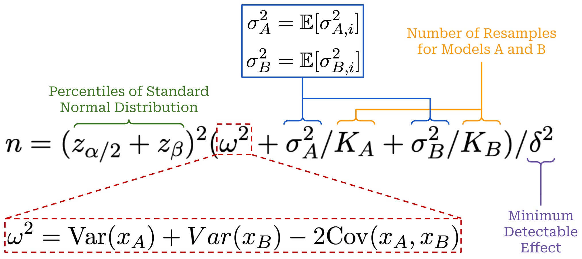
This sample size formula provides useful intuition for statistical significance in LLM evaluations. Our evaluation requires a larger sample size when:
The amount of variance is large.
The size of the effect being detected is small.
A stricter confidence or higher level of power is desired.
Additionally, we can decrease the necessary value of n by performing resampling, revealing that our previously-outlined techniques for variance reduction are still applicable. Notably, the sample size also grows quadratically with the inverse of the minimum detectable effect: detecting a gap in performance that is half the size requires 4× the number of samples. We can also rearrange this sample size equation to solve for the minimum detectable effect δ, allowing us to determine the smallest gap in performance that can be detected with some benchmark.
Sample size implementation. To compute the above sample size formula, we must solve for the correct z_p values given a specified significance level α and power 1 - β, as well as estimate the three variance terms from actual evaluation data. An example implementation is provided below for reference, which adopts the same patterns as our evaluation statistics code from the prior section.
import math
import numpy as np
from statistics import NormalDist


##########################
# Power analysis settings
##########################

alpha = 0.05
beta = 0.20
delta = 0.10


#################################
# Model scores (three resamples)
#################################

model_a_scores = np.array([
    [1, 1, 1],
    [0, 1, 0],
    [1, 1, 0],
    [1, 1, 1],
    [0, 0, 0],
    [1, 1, 1],
    [1, 0, 1],
    [0, 0, 1],
    [1, 1, 1],
    [1, 0, 1],
], dtype=float)

model_b_scores = np.array([
    [1, 0, 1],
    [0, 0, 0],
    [1, 0, 0],
    [1, 0, 1],
    [0, 0, 0],
    [1, 1, 0],
    [0, 0, 1],
    [0, 0, 0],
    [1, 0, 1],
    [1, 0, 0],
], dtype=float)


##########################################
# Compute z_p values from alpha and beta
#
# The paper uses:
# - z_{alpha/2}
# - z_beta, where power = 1 - beta
##########################################

def z_alpha_over_2(alpha: float) -> float:
    return NormalDist().inv_cdf(1 - alpha / 2)

def z_beta(beta: float) -> float:
    return NormalDist().inv_cdf(1 - beta)


#####################################
# Sample estimates of variance terms
#####################################

def question_means(score_matrix: np.ndarray) -> np.ndarray:
    """
    Estimate x_i for each question i by averaging over K samples.
    """
    return np.mean(score_matrix, axis=1)

def question_conditional_variances(score_matrix: np.ndarray) -> np.ndarray:
    """
    Estimate sigma_i^2 for each question i using the within-question
    sample variance across repeated samples. We cannot estimate this
    if we only have 1 resample (i.e., K = 1).
    """
    n, k = score_matrix.shape
    if k == 1:
        return np.zeros(n)
    return np.var(score_matrix, axis=1, ddof=1)

def estimate_sigma_squared(score_matrix: np.ndarray) -> float:
    """
    Estimate E[sigma_i^2] by averaging the within-question variances.
    """
    return float(np.mean(question_conditional_variances(score_matrix)))

def estimate_omega_squared(
    model_a_score_matrix: np.ndarray,
    model_b_score_matrix: np.ndarray,
) -> float:
    """
    Estimate:

        omega^2 = Var(x_A) + Var(x_B) - 2 Cov(x_A, x_B) = Var(x_A - x_B)

    where x_A and x_B are the question-level conditional means using sample
    variance and covariance across questions.
    """
    x_a = question_means(model_a_score_matrix)
    x_b = question_means(model_b_score_matrix)

    # compact form is Var(x_A - x_B)
    # equivalent to Var(x_A) + Var(x_B) - 2 Cov(x_A, x_B)
    """
    Expanded version:
    var_a = np.var(x_a, ddof=1)
    var_b = np.var(x_b, ddof=1)
    cov_ab = np.cov(x_a, x_b, ddof=1)[0, 1]
    return float(var_a + var_b - 2 * cov_ab)
    """
    diffs = x_a - x_b
    return float(np.var(diffs, ddof=1))

def estimate_power_analysis_variance_terms(
    model_a_score_matrix: np.ndarray,
    model_b_score_matrix: np.ndarray,
) -> dict:
    """
    Estimate all variance terms needed for sample-size formula in [1].
    """
    sigma_a_sq = estimate_sigma_squared(model_a_score_matrix)
    sigma_b_sq = estimate_sigma_squared(model_b_score_matrix)
    omega_sq = estimate_omega_squared(model_a_score_matrix, model_b_score_matrix)

    n_questions, k_a = model_a_score_matrix.shape
    n_questions_b, k_b = model_b_score_matrix.shape

    return {
        "n_questions": n_questions,
        "K_A": k_a,
        "K_B": k_b,
        "omega_sq": omega_sq,
        "sigma_a_sq": sigma_a_sq,
        "sigma_b_sq": sigma_b_sq,
    }


###############################
# Sample size formula from [1]
###############################

def required_sample_size(
    delta: float,
    alpha: float,
    beta: float,
    omega_sq: float,
    sigma_a_sq: float,
    sigma_b_sq: float,
    K_A: int = 1,
    K_B: int = 1,
) -> float:
    z_a2 = z_alpha_over_2(alpha)
    z_b = z_beta(beta)

    variance_term = omega_sq + sigma_a_sq / K_A + sigma_b_sq / K_B
    n = ((z_a2 + z_b) ** 2 * variance_term) / (delta ** 2)
    return float(n)


################################
# Compute Sample Size
################################

def main():
    terms = estimate_power_analysis_variance_terms(model_a_scores, model_b_scores)

    print("=" * 80)
    print("Estimated variance terms from fixed evaluation results")
    print("=" * 80)
    print(f"n_questions = {terms['n_questions']}")
    print(f"K_A = {terms['K_A']}")
    print(f"K_B = {terms['K_B']}")
    print(f"omega^2 = {terms['omega_sq']:.6f}")
    print(f"sigma_A^2 = {terms['sigma_a_sq']:.6f}")
    print(f"sigma_B^2 = {terms['sigma_b_sq']:.6f}")
    print()

    print("=" * 80)
    print("Critical z-values")
    print("=" * 80)
    print(f"alpha = {alpha:.3f}")
    print(f"beta  = {beta:.3f}")
    print(f"power = {1 - beta:.3f}")
    print(f"z_(alpha/2) = {z_alpha_over_2(alpha):.6f}")
    print(f"z_beta      = {z_beta(beta):.6f}")
    print()

    n_required = required_sample_size(
        delta=delta,
        alpha=alpha,
        beta=beta,
        omega_sq=terms["omega_sq"],
        sigma_a_sq=terms["sigma_a_sq"],
        sigma_b_sq=terms["sigma_b_sq"],
        K_A=terms["K_A"],
        K_B=terms["K_B"],
    )

    print("=" * 80)
    print("Required sample size")
    print("=" * 80)
    print(f"Target effect size delta = {delta:.4f}")
    print(f"Required n ≈ {n_required:.2f}")
    print()

main()
Don’t Use the CLT in LLM Evals With Fewer Than a Few Hundred Datapoints [2]
“Assumptions underlying the asymptotic, CLT-based approaches may not be suitable for LLM evals, at least in smaller data regimes. In that case, we expect to see broader failures of CLT-based confidence intervals.” - from [2]
In [2], authors extend the proposals from [1] by analyzing the effectiveness of the CLT in the small data regime (i.e., n <= 100). As we have learned, the CLT implies that sample means approach a normal distribution as the sample size n increases, but the value of n may have to be in the hundreds or thousands for this property to hold—the point at which n becomes “big enough” is difficult to determine a priori. The key insight from [2] is that the CLT underestimates uncertainty when there is limited evaluation data. This problem is worsened by the fact that LLM benchmarks are becoming increasingly specialized, leading many to the creation of many smaller benchmarks that capture performance on particular tasks (e.g., the popular SWE-Bench Verified benchmark contains only 500 questions).
CLT simulations. The shortcomings of the CLT are demonstrated in [2] via extensive simulation experiments with a known ground truth that permit directly verifying a confidence interval. From these simulations, we see that CLT-based methods consistently fail in small-data regimes by producing confidence intervals that are too narrow and overly-confident. Several scenarios are considered in the simulations in [2] that mostly align with evaluation setups from [1]:
IID questions: model performance is measured on IID questions (assumed to be binary in [2]).
Clustered questions: model performance is analyzed on questions that are not IID (i.e., the clustered setting from [1]).
Unpaired model comparison: model performance is measured over separate question sets and compared between models.
Paired model comparison: model performance is measured on an identical set of questions and compared between models.
Across all settings, evidence presented against CLT-based methods in the small n regime is clear—the CLT fails across all scenarios when n < 100. Such findings emphasize the fact that the CLT, despite being simple and powerful, makes underlying assumptions (i.e., IID variables, finite variance, and sufficiently large n) that degrade its effectiveness when violated. Authors in [2] do not recommend against using the CLT. Rather, they encourage awareness of these assumptions and limitations so that the CLT can be avoided in situations where it does not apply. Specifically, the key failure case for the CLT in [2] is when n < 100.
“It may be argued that CLT-based methods are usually sufficient in practice when their assumptions are satisfied. We do not disagree. However, we argue that it is safer to use the more robust strategies laid out in this paper, which are just as easy to apply, perform no worse for large n and perform substantially better in the small-n setting… knowing whether a certain n is large enough for the CLT to hold would be extremely context-dependent and difficult to determine a priori.” - from [2]
One other specific issue highlighted with the CLT in [2] is cases where models begin to achieve either perfect or zero accuracy. On especially small datasets, it is possible that an LLM either answers all questions correctly or—in the case of a tiny but non-trivial dataset like AIME—answers no questions correctly. In these cases, confidence intervals produced with the CLT will become overly narrow because all scores are the same, thus worsening issues with overconfidence.
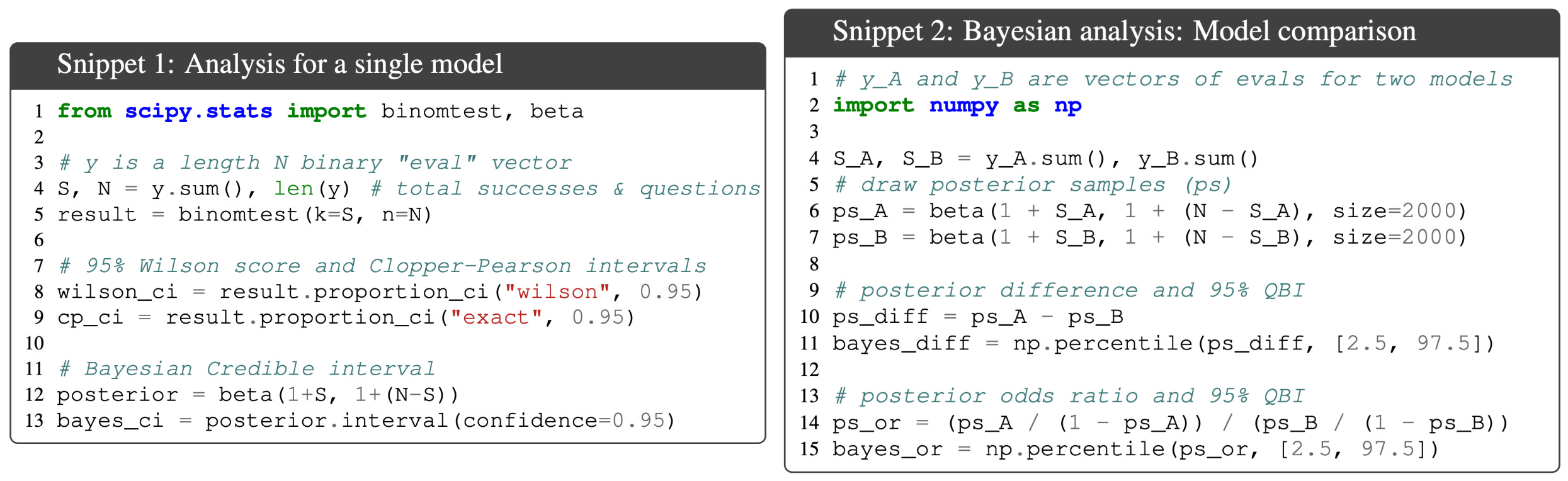
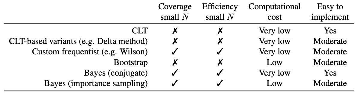
Alternative approaches. Although the full details of these techniques are beyond the scope of this post, authors in [2] provide several possible alternative methods for computing confidence intervals. Most prominent among these techniques are Bayesian methods, which are less sensitive to the value of n and can provide narrower confidence intervals relative to the CLT. As shown above, Bayesian intervals are still relatively straightforward to compute and can be extended to handle important settings such as clustered questions or model comparisons. A brief overview of several alternative techniques—including Bayesian methods—alongside their benefits and drawbacks is provided below for reference.
Quantifying Variance in Evaluation Benchmarks [3]
“If we cannot trust our evaluation results or do not understand what improvements are statistically significant, we cannot make sound comparisons, making it more challenging to reliably use benchmarks.” - from [3]
As we have learned, most LLM evaluations just report a single deterministic score (e.g., an accuracy of 70% on MMLU) without explicitly accounting for variability. Small score differences are often used to claim superior performance of a model, but it is usually unclear whether a small difference is attributable to noise or actually a meaningful capability improvement. This issue causes misleading or even incorrect results on benchmarks, as well as poor decision making during the model development process. In [3], authors perform a deep dive into variance of LLM evaluation using 13 popular benchmarks and over 280 models.
Measuring variability. In order to perform a large-scale analysis of benchmark variance, a broad group of LLMs is curated in [3]. First, a group of seed models—all based upon Llama-2-7B—is created by training from scratch with different random initialization seeds on 210 billion tokens of data. Checkpoints are collected throughout training for each seed, resulting in 210 total snapshots that are used for evaluation. These seed models are then supplemented with an additional 41 checkpoints of Llama 1 and 2 from various training stages, as well as 32 other models across a variety of families (e.g., Gemma and Mistral). This group of models is then evaluated over a set of 13 benchmarks that cover a wide variety of domains like reasoning, math, general knowledge, and coding.
Variance metrics. To study the variability in evaluation results, three metrics are considered in [3]:
Seed variance measures the standard deviation of performance across models trained with different random seeds and is reported as an average over all training checkpoints.
Monotonicity8 measures the whether the sequence of evaluation scores for a model improve regularly throughout training.
The signal-to-noise ratio (SNR) of seed models is measured by dividing the mean benchmark score of the final model across different seeds by the standard deviation of scores across seeds.
Key findings. We learn in [1] that different benchmarks have drastically different variance characteristics; see below. For example, smaller benchmarks (e.g., COPA and HumanEval) are found to have higher seed variance and larger confidence intervals, emphasizing once again the need for evaluation datasets that are sufficiently large. Additionally, some benchmarks have random performance for smaller models, even after extensive training. These benchmarks may be too difficult for certain models, which reflects findings in current research showing that certain benchmarks may only be useful at a specific scale.
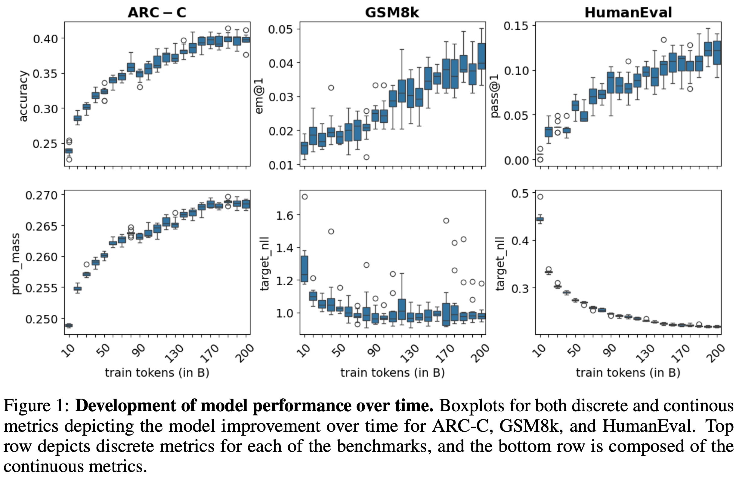
We also see in [3] that using a continuous evaluation formulation based upon token probabilities yields more reliable evaluation results compared to binary evaluations based upon correctness. Notably, this finding aligns with the variance reduction analysis provided in [1]. Specifically, authors in [3] compute continuous metrics using either:
The probability of the correct answer token for multiple choice questions.
The log likelihood of a reference answer—computed by summing the log probabilities for all tokens in a completion—for open-ended generations.
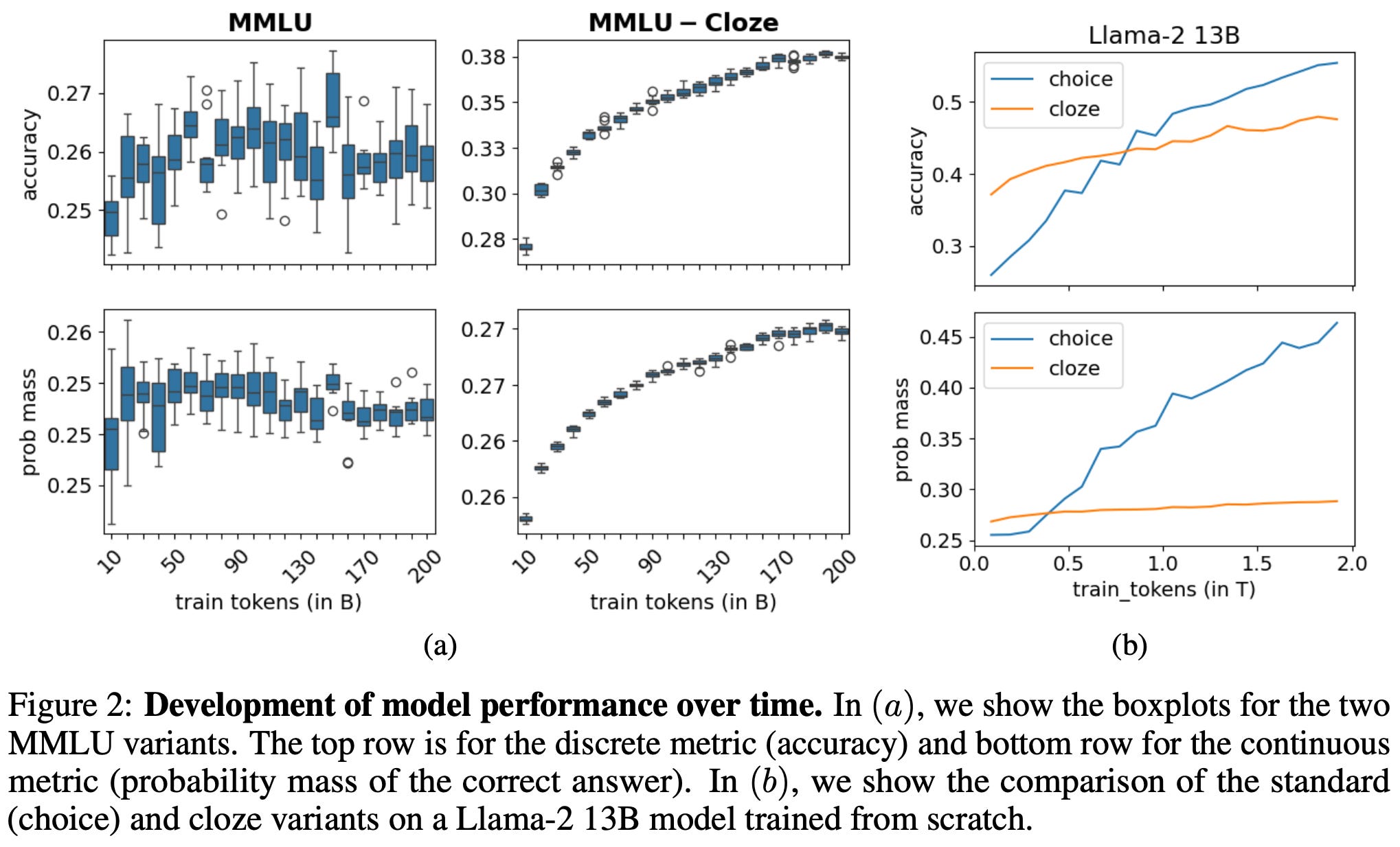
By using continuous evaluation metrics based upon these token probabilities, the SNR and monotonicity of evaluation benchmarks noticeably improve; see above. Based upon this observation, authors in [3] also reformulate the popular MMLU question-answering benchmark to be completion-based instead of using multiple choice questions—this new dataset is called MMLU-Cloze9. As shown in the figure below, this reformulation drastically reduces the variability of the benchmark, thus highlighting the benefit of using continuous metrics for LLM evaluation.
Signal and Noise: A Framework for Reducing Uncertainty in Language Model Evaluation [4]
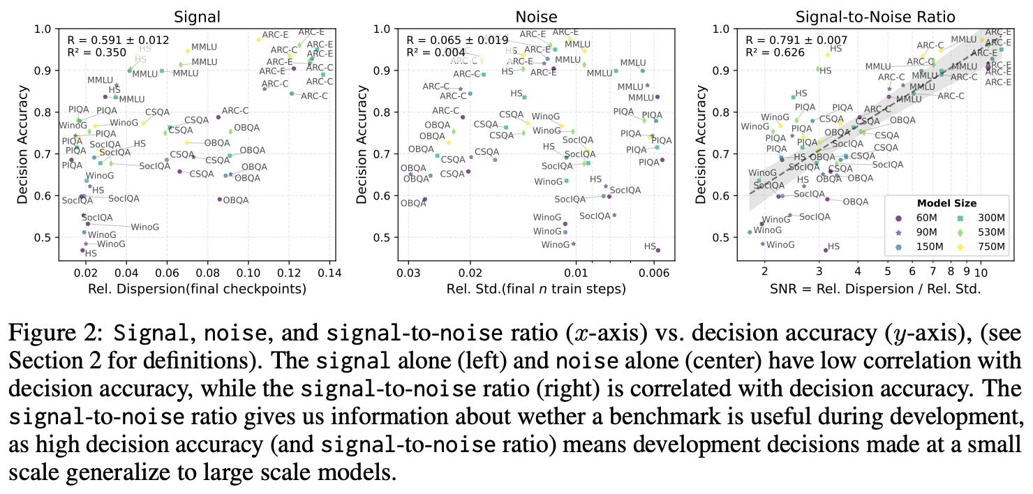
During the LLM development process, we perform small-scale experiments to tune our training settings and rely upon evaluation results to determine the best setting. However, the results of small-scale experiments may not translate well to large-scale training runs, and noise in the evaluation process can lead to incorrect decisions. In [4], an SNR-based framework is proposed for assessing benchmark reliability and improving the predictive accuracy of evaluation across scales.
Assessing reliability. Evaluation datasets are analyzed in [4] using an SNR metric, but a specific definition of signal and noise is proposed. Assume scores is an array of scores for a benchmark, where each index stores the evaluation score for a different model. We define signal = [max(scores) - min(scores)] / mean(scores). In other words, the signal metric captures the relative spread of scores across models for a particular benchmark.
Noise measures variability in performance due to randomness in the training process. To compute noise, we could train multiple models with different random seeds and measure the variance in their evaluation scores. However, such an approach is computationally expensive. As a solution, noise is measured in [4] by:
Considering the last
nmodel checkpoints from the training process.Obtaining the evaluation result for each of these checkpoints, yielding a list of evaluation scores
ckpt_scores.Computing
noise = std(ckpt_scores) / mean(ckpt_scores).
We can then combine these metrics into a single SNR metric by taking the quotient of signal and noise. This SNR metric is helpful for analyzing benchmark reliability, as any evaluation dataset with high SNR is capable of distinguishing between different models and is relatively insensitive to training randomness.
Practical tips. The SNR metric is validated in a large-scale evaluation study in [4] that considers 465 LLMs and 30 evaluation benchmarks. Across all evaluation settings, we see that benchmarks with higher SNR provide more reliable model rankings. Specifically, the correlation between SNR and decision accuracy—meaning that the better model receives a higher evaluation score on a particular benchmark—is found to be quite high. Several practical tips for LLM evaluations are proposed in [4] based on these observations:
For an evaluation benchmark, we can select specific sub-tasks with the highest SNR to improve reliability. For example, authors in [4] use SNR to select 16 (of 57 total) MMLU tasks for evaluation, which improves decision accuracy and drastically reduces evaluation costs.
Instead of only evaluating the final model checkpoint, we can compute an average evaluation score across the last
nmodel checkpoints to improve reliability and mitigate noise due to training randomness.
Authors in [4] also advocate for using continuous—rather than discrete—metrics for evaluation. Similarly to findings in [1, 3], we see in [4] that evaluating a model based upon the log likelihood of the correct completion improves the reliability of the evaluation process, as evidenced by a clearly-improved SNR.
“We calculate the bits-per-byte (BPB) using the correct continuations of each test set. The bits-per-byte is the negative log likelihood of the correct answer divided by the number of UTF-8 bytes in the answer string.” - from [4]
Key Takeaways
In this overview, we have learned a wide variety of tools for evaluating LLMs in an uncertainty-aware manner. To close, we will summarize what we’ve learned by outlining how each of these tools can be used when evaluating an LLM. In the simplest case, we can draw upon the CLT to derive a standard error and confidence interval along with our evaluation results. However, there are a few cases in which this approach will not yield valid results:
If the value of
nis small, then the CLT-based standard error expression is overly confident. We can solve this issue by evaluating over a larger dataset or using another approach (e.g., the Bayesian methods outlined in [2]) that is better equipped to deal with smallern.If evaluation questions are not independent, then we can derive a cluster-adjusted standard error to account for the relationship between questions in our evaluation dataset.
When comparing models that are evaluated on the same questions (i.e., a paired setup), we can apply the same approaches over their question-level differences to provide a more statistically efficient estimate of which model performs better.
To reduce evaluation variance, we can use resampling, where K is selected such that E[σ_i^2 / K] ≪ Var(X). In some settings, token probabilities can be used to compute the expected score—or the probability of the ground truth answer— directly, thus reducing within-question variance. Such an approach has been shown in several concurrent works [1, 3, 4] to improve the stability of evaluation results. When creating an evaluation dataset, we can use power analysis—or just adopt the sample size formula from [1]—to determine the number of samples needed. We can also rearrange the sample size formula to find the minimum detectable effect δ that can be measured with a given dataset, which helps us to determine whether certain evaluations are even worth running at all.
New to the newsletter?
Hi! I’m Cameron R. Wolfe, Deep Learning Ph.D. and Senior Research Scientist at Netflix. This is the Deep (Learning) Focus newsletter, where I help readers better understand important topics in AI research. The newsletter will always be free and open to read. If you like the newsletter, please subscribe, consider a paid subscription, share it, or follow me on X and LinkedIn!
Bibliography
[1] Miller, Evan. “Adding error bars to evals: A statistical approach to language model evaluations.” arXiv preprint arXiv:2411.00640 (2024).
[2] Bowyer, Sam, Laurence Aitchison, and Desi R. Ivanova. “Position: Don’t Use the CLT in LLM Evals With Fewer Than a Few Hundred Datapoints.” arXiv preprint arXiv:2503.01747 (2025).
[3] Madaan, Lovish, et al. “Quantifying variance in evaluation benchmarks, 2024.” URL https://arxiv. org/abs/2406.10229 (2024).
[4] Heineman, David, et al. “Signal and noise: A framework for reducing uncertainty in language model evaluation.” arXiv preprint arXiv:2508.13144 (2025).
The evaluation process is stochastic, so if we re-run the evaluation on this question multiple times we can observe a different result!
Previously, we introduced the sample variance, denoted as s^2. The sample standard deviation, denoted as s, is simply the square root of this expression.
The z-score refers to the realized value z of the random variable Z.
The reason we must assume variance σ^2 is finite is so that this expression is well-defined and exists. The standard deviation and standard error are not finite or meaningful when variance is infinite.
We write the normal distribution as N(x, y), where x is the mean of the normal distribution and y is the variance.
Here, the unconditional versions of s and x (i.e., without the i subscript) is used, so we are taking this expectation over the entire super-population.
More specifically, if we are reporting a metric in the range [0, 1] (e.g., an f1 score), then this formula cannot be used. These are fractional scores rather than binary scores with a value of either 0 or 1.
Practically, monotonicity is computed by taking the sequence of scores throughout training and measuring the Kendall rank correlation between this sequence and a perfectly monotonic sequence (i.e., a sequence in which the model’s performance increases at every checkpoint throughout training).
In the context of LLMs, a Cloze task refers to a fill-in-the-blank test where the LLM is given context (e.g., a paragraph or sentence) with missing tokens and expected to predict the missing information.
For agent evals, should we consider prompts that share the same environment (a code repo, a synthetic database, etc.) as dependent and in the same cluster? What would that mean for a set of agent evals that all share the same environment, like the agent company, as an example
Thank You for writing this. Much needed. I think soon we'll be in the Era of some substack posts getting more Citations than papers. This might be one of those.