Basics of Reinforcement Learning for LLMs
Understanding the problem formulation and basic algorithms for RL..
Recent AI research has revealed that reinforcement learning—more specifically, reinforcement learning from human feedback (RLHF)—is a key component of training a state-of-the-art large language model (LLM). Despite this fact, most open-source research on language models heavily emphasizes supervised learning strategies, such as supervised fine-tuning (SFT). This lack of emphasis upon reinforcement learning can be attributed to several factors, including the necessity to curate human preference data or the amount of data needed to perform high-quality RLHF. However, one undeniable factor that likely underlies skepticism towards reinforcement learning is the simple fact that it is not as commonly-used compared to supervised learning. As a result, AI practitioners (including myself!) avoid reinforcement learning due to a simple lack of understanding—we tend to stick with using the approaches that we know best.
“Many among us expressed a preference for supervised annotation, attracted by its denser signal… However, reinforcement learning proved highly effective, particularly given its cost and time effectiveness.” - from [8]
This series. In the next few overviews, we will aim to eliminate this problem by building a working understanding of reinforcement learning from the ground up. We will start with basic definitions and approaches—covered in this overview—and work our way towards modern algorithms (e.g., PPO) that are used to finetune language models with RLHF. Throughout this process, we will explore example implementations of these ideas, aiming to demystify and normalize the use of reinforcement learning in the language modeling domain. As we will see, these ideas are easy to use in practice if we take the time to understand how they work!
What is Reinforcement Learning?
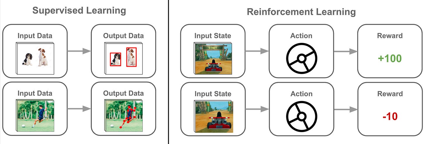
At the highest level, reinforcement learning (RL) is just another way of training a machine learning model. In prior overviews, we have seen a variety of techniques for training neural networks, but the two most commonly-used techniques for language models are supervised and self-supervised learning.
(Self-)Supervised Learning. In supervised learning, we have a dataset of inputs (i.e., a sequence of text) with corresponding labels (e.g., a classification or completion of the input text), and we want to train our model to accurately predict those labels from the input. For example, maybe we want to finetune a language model (e.g., BERT) to classify sentences that contain explicit language. In this case, we can obtain a dataset of sentences with binary labels indicating whether the sentence contains explicit language or not. Then, we can train our language model to classify this data correctly by iteratively:
Sampling a mini-batch of data from the dataset.
Predicting the labels with the model.
Computing the loss (e.g., CrossEntropy).
Backpropagating the gradient through the model.
Performing a weight update.
Self-supervised learning is similar to the setup explained above, but there are no explicit labels within our dataset. Rather, the “labels” that we use are already present within the input data. For example, language models are pretrained with a self-supervised language modeling objective that trains the model to predict the next token given prior tokens as input. Here, the next token is already present within the data (assuming that we have access to the full textual sequence1).
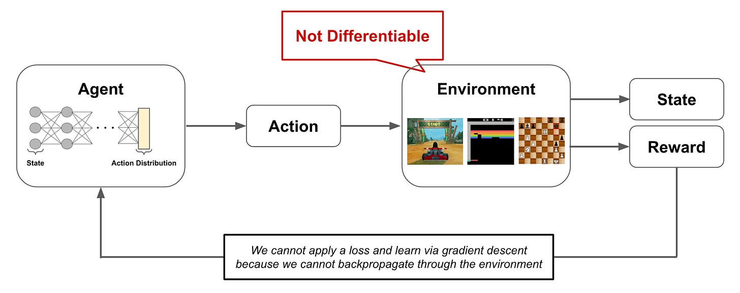
When is RL useful? Although RL is just another way of training a neural network, the training setup is different compared to supervised learning. Similarly to how humans learn, RL trains neural networks through trial and error. More specifically, the neural network will produce an output, receive some feedback about this output, then learn from the feedback. For example, when finetuning a language model with reinforcement learning from human feedback (RLHF), the language model produces some text then receives a score/reward from a human annotator2 that captures the quality of that text; see above. Then, we use RL to finetune the language model to generate outputs with high scores.
In this case, we cannot apply a loss function that trains the language model to maximize human preferences with supervised learning. Why? Well, the score that we get from the human is a bit of a black box. There’s no easy way for us to explain this score or connect it mathematically to the output of the neural network. In other words, we cannot backpropagate a loss applied to this score through the rest of the neural network. This would require that we are able to differentiate (i.e., compute the gradient of) the system that generates the score, which is a human that subjectively evaluates the generated text; see above.
Big picture. The above discussion starts to provide us with insight as to why RL is such a beautiful and promising learning algorithm for neural networks. RL allows us to learn from signals that are non-differentiable and, therefore, not compatible with supervised learning. Put simply, this means that we can learn from arbitrary feedback on a neural network’s output! In the case of RLHF, we can score the outputs generated by a language model according to any principle that we have in mind. Then, we can use RL to learn from these scores, no matter how we choose to define them! In this way, we can teach a language model to be helpful, harmless, honest, more capable (e.g., by using tools), and much more.
A Formal Framework for RL
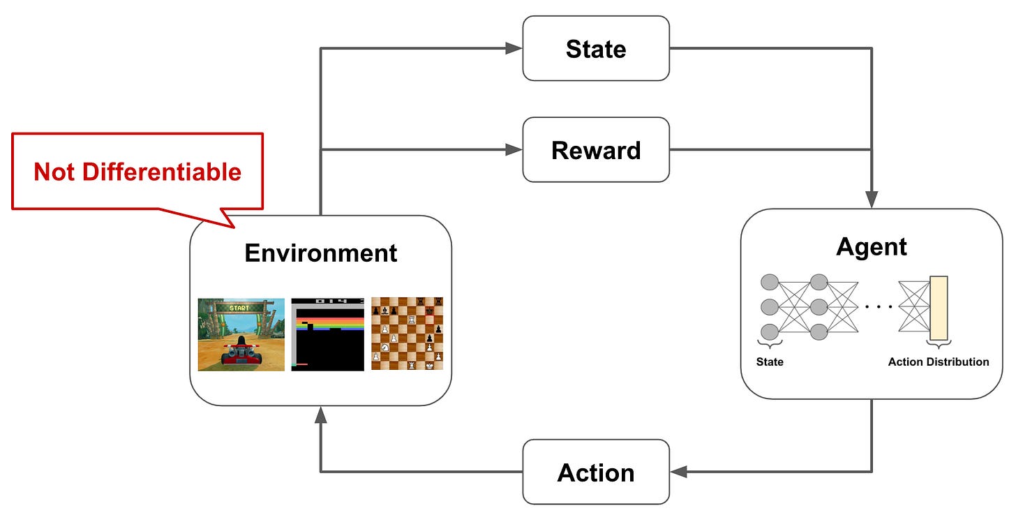
Problems that are solved via RL tend to be structured in a similar format. Namely, we have an agent that is interacting with an environment; see above. The agent has a state in the environment and produces actions, which can modify the current state, as output. As the agent interacts with the environment, it can receive both positive and negative rewards for its actions. The agent’s goal is to maximize the rewards that it receives, but there is not a reward associated with every action taken by the agent! Rather, rewards may have a long horizon, meaning that it takes several correct, consecutive actions to generate any positive reward.
Markov Decision Process (MDP)
To make things more formal and mathematically sound, we can formulate the system described above as a Markov Decision Process (MDP). Within an MDP, we have states, actions, rewards, transitions, and a policy; see below.
States and actions have discrete values, while rewards are real numbers. In an MDP, we define two types of functions: transition and policy functions. The policy takes a state as input3, then outputs a probability distribution over possible actions. Given this output, we can make a decision for the action to be taken from a current state, and the transition is then a function that outputs the next state based upon the prior state and chosen action. Using these components, the agent can interact with the environment in an iterative fashion; see below.
One thing we might be wondering here is: What is the difference between the agent and the policy? The distinction is a bit nuanced. However, we can think of the agent as implementing the policy within its environment. The policy describes how the agent chooses its next action given the current state. The agent follows this strategy as it interacts with the environment, and our goal is to learn a policy that maximizes the reward that the agent receives from the environment.
As the agent interacts with the environment, we form a “trajectory” of states and actions that are chosen throughout this process. Then, given the reward associated with each of these states, we get a total return given by the equation below, where γ is the discount factor (more explanation coming soon). This return is the summed reward across the agent’s full trajectory, but rewards achieved at later time steps are exponentially discounted by the factor γ; see below.
The goal of RL is to train an agent that maximizes this return. As shown by the equation below, we can characterize this as finding a policy that maximizes the return over trajectories that are sampled from the final policy4.
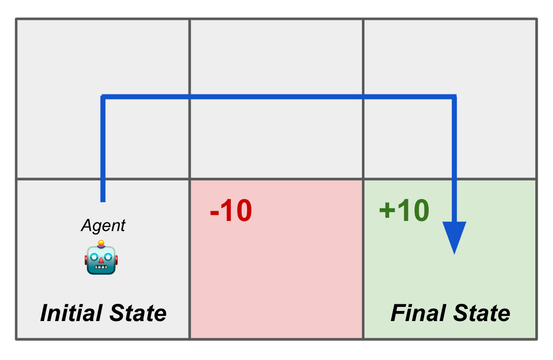
Example application. As a simplified example of the setup described above, let’s consider training a neural network to navigate a 2 X 3 grid from some initial state to some final state; see below. Here, we see in the grid that the agent will receive a reward of +10 for reaching the desired final state and a reward of -10 whenever it visits the red square.
Our environment is the 2 X 3 grid and the state is given by the current position within this grid—we can represent this as a one-hot vector. We can implement our policy with a feed-forward neural network5 that takes the current one-hot position as input and predicts a probability distribution over potential actions (i.e., move up, move down, move left, move right). For each chosen action, the transition function simply moves the agent to the corresponding next position on the grid and avoids allowing the agent to move out of bounds. The optimal agent learns to reach the final state without passing through the red square; see below.
Like many problems that are solved with RL, this setup has an environment that is not differentiable (i.e., we can’t compute a gradient and train the model in a supervised fashion) and contains long-term dependencies, meaning that we might have to learn how to perform several sequential actions to get any reward.
Great… but how does this apply to language models? The application described above is a traditional use case for RL, including an agent/policy that learns to interact with an external (potentially simulated) environment. There are numerous examples of such successful applications of RL; e.g., Atari [3], Go, autonomous driving [4] and more. However, RL has recently been leveraged for finetuning language models. Although this is a drastically different use case, the components discussed above can be easily translated to language modeling!
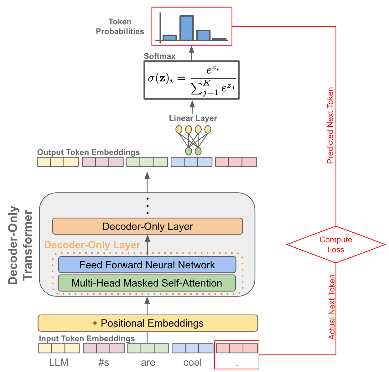
As has been discussed extensively in prior overviews, language models specialize in performing next token prediction; see above. In other words, our language model takes several tokens as input (i.e., a prefix) and predicts the next token based on this context. When generating text at inference time, this is done autoregressively, meaning that the language model continually:
Predicts the next token.
Adds the next token to the current input sequence.
Repeats.
To view this setup from the lens of RL, we can consider our language model to be the policy. Our state is just the current textual sequence. Given this state as input, the language model can produce an action—the next token—that modifies the current state to produce the next state—the textual sequence with an added token. Once a full textual sequence has been produced, we can obtain a reward by rating the quality of the language model’s output, either with a human or a reward model that has been trained over human preferences.
Although this setup is quite different from learning to navigate a simple grid (i.e., the model, data modality, environment, and reward function are all completely different!), we begin to see that the problem formulation used for RL is quite generic. There are many different problems that we can solve using this approach!
Important Terms and Definitions
Now that we understand the basic setup that is used for RL, we should overview some of the common terms we might see when studying this area of research. We have outlined a few notable terms and definitions below.
Trajectory: A trajectory is simply a sequence of states and actions that describe the path taken by an agent through an environment.
Episode: Sometimes, the environment we are exploring has a well-defined end state; e.g., reaching the final destination in our 2 X 3 grid. In these cases, we refer to the trajectory of actions and states from start to end state as an episode.
Return: Return is just the reward summed over an entire trajectory. As shown above, however, this sum typically includes a discount factor. Intuitively, this means that current rewards are more valuable than later rewards, due to both uncertainty and the simple fact that waiting to receive a reward is less desirable.
Discount factor: The concept of discounting goes beyond RL (e.g., discounting is a core concept in finance) and refers to the basic idea of determining the current value of a future reward. As shown by the equation above, we handle discounting in RL via an exponential6 discount factor. Although the intuitive explanation of the discount factor is easy to understand, the exact formulation we see above is rooted in mathematics and is actually a complex topic of discussion; see below.
On vs. Off-Policy: In RL, we have a target policy that describes the policy our agent is aiming to learn. Additionally, we have a behavior policy that is being used by the agent to select actions as it interacts with the environment. The distinction between on and off-policy learning is subtle, but the difference between these two approaches lies in whether the behavior policy used to select actions as the agent navigates the environment during RL is the same (on-policy) as the target policy that we are trying to evaluate and improve or not (off-policy).
ε-Greedy Policy: RL trains a neural network via interaction with an environment. The policy that this neural network implements takes a current state as input and produces a probability distribution over potential actions as output. But, how do we choose which action to actually execute? One of the most common approaches is an ε-greedy policy, which selects the action with the highest expected return most of the time (i.e., with probability 1 - ε) and a random action otherwise. Such an approach balances exploration and exploitation by allowing the agent to explore new actions in addition to those that it knows to work well.
Q-Learning: A Simple Introduction to RL
Now that we understand the framework that is typically used to solve problems with RL, let’s take a look at our first RL algorithm. This algorithm, called Q-Learning, is simple to understand and a great intro into the topic. Once we understand Q-Learning, we will also study our first deep RL algorithm (i.e., a system that trains a deep neural network with RL), called Deep Q-Learning.
Q-Learning: Modeling Q Values with a Lookup Table
Q-Learning is a model-free RL algorithm, meaning that we don’t have to learn a model for the environment with which the agent interacts. Concretely, this means that we don’t have to train a model to estimate the transition or reward functions—these are just given to us as the agent interacts with the environment. The goal of Q-Learning is to learn the value of any action at a particular state. We do this through learning a Q function, which defines the value of a state-action pair as the expected return of taking that action at the current state under a certain policy and continuing afterwards according to the same policy.
To learn this Q function, we create a lookup table for state-action pairs. Each row in this table represents a unique state, and each column represents a unique action; see above. The values within each of entry of the lookup table represent the Q value (i.e., the output of the Q function) for a particular state-action pair. These Q values are initialized as zero and updated—using the Bellman equation—as the agent interacts with the environment until they become optimal.
The algorithm. The first step of Q-learning is to initialize our Q values as zero and pick an initial state with which to start the learning process. Then, we iterate over the following steps (depicted above):
Pick an action to execute from the current state (using an ε-Greedy Policy).
Get a reward and next state from the (model-free) environment.
Update the Q value based on the Bellman equation.
As shown in the figure above, our update to the Q value considers the reward of the current action, the Q value of the current state, and the Q value of the next state. However, given that our agent might execute several actions within the next state, it is unclear which Q value we should use for the next state when performing our update. In Q-learning, we choose to use the maximum Q value, as shown below.
Interestingly, Q-learning utilizes an ε-greedy policy when selecting actions, allowing new states and actions to be explored with a certain probability. When computing Q value updates, however, we always consider the next action with the maximum Q value, which may or may not be executed from the next state. In other words, Q-learning estimates the return for state-action pairs by assuming a greedy policy that just selects the highest-return action at the next state, even though we don’t follow such an approach when actually selecting an action. For this reason, Q-learning is an off-policy learning algorithm; see here for more details.
Brief mathematical note. The update rule used for Q-learning is mathematically guaranteed to find an optimal policy for any (finite) MDP—meaning that we will get a policy that maximizes our objective given sufficient iterations of the above process. An approachable and (almost) self-contained proof of this result is provided in [5].
Deep Q-Learning
The foundation of Deep Q-learning (DQL) lies in the vanilla Q-learning algorithm described above. DQL is just an extension of Q-learning for deep reinforcement learning, meaning that we use an approach similar to Q-learning to train a deep neural network. Given that we are now using a more powerful model (rather than a lookup table), Deep Q-Learning can actually be leveraged in interesting (but still relatively simple) practical applications. Let’s take a look at this algorithm and a few related applications that might be of interest.

The problem with Q-Learning. The size of the lookup table that we define for Q-learning is dependent upon the total number of states and actions that exist within an environment. In complex environments (e.g., high-resolution video games or real life), maintaining such a lookup table is intractable—we need a more scalable approach. DQL solves this problem by modeling the Q function with a neural network instead of a lookup table; see above. This neural network takes the current state as input and predicts the Q values of all possible actions from that state as output. DQL eliminates the need to store a massive lookup table! We just store the parameters of our neural network and use it to predict Q values.
The algorithm. In DQL, we have two neural networks: the Q network and the target network. These networks are identical, but the exact architecture they use depend upon the problem being solved7. To train these networks, we first gather data by interacting with the environment. This data is gathered using the current Q network with an ε-greedy policy. This process of gathering interaction data for training the Q network is referred to as experience replay; see above.
From here, we use data that has been collected to train the Q network. During each training iteration, we sample a batch of data and pass it through both the Q network and the target network. The Q network takes the current state as input and predicts the Q value of the action that is taken (i.e., predicted Q value), while the target network takes the next state as input and predicts the Q value of the best action that can be taken from that state8 (i.e., target Q value).
From here, we use the predicted Q value, the target Q value, and the observed reward to train the Q network with an MSE loss; see above. The target network is held fixed. Every several iterations, the weights of the Q network are copied to the target network, allowing this model to be updated as well. Then, we just repeat this process until the Q network converges. Notably, the dataset we obtain from experience replay is cumulative, meaning that we maintain all of the data we have observed from the environment throughout all iterations.
Why do we need the target network? The vanilla Q-learning framework leverages two Q values in its update rule: a (predicted) Q value for the current state-action pair and the (target) Q value of the best state-action pair for the next state. In DQL, we similarly have to generate both of these Q values. In theory, we could do this with a single neural network by making multiple passes through the Q network—one for the predicted Q value and one for the target Q value. However, the Q network’s weights are being updated at every training iteration, which would cause the target Q value to constantly fluctuate as the model is updated. To avoid this issue, we keep the target network separate and fixed, only updating its weights every several iterations to avoid creating a “moving target”.
This idea of using a separate network to produce a training target for another network—referred to as knowledge distillation [6]—is heavily utilized within deep learning. Furthermore, the idea of avoiding too much fluctuation in the weights of the teacher/target model has been addressed in this domain. For example, the mean teacher approach [7] updates the weights of the teacher model as an exponential moving average of the student network’s weights; see above. In this way, we can ensure a stable target is provided by the teacher during training.
Practical applications. DQL is a deep RL framework that has been used for several interesting practical applications. One early and notable demonstration of DQL was for playing Atari breakout. In [3], authors from Google DeepMind show that Deep Q-Learning is a useful approach for training a agents that can successfully beat simple video games. For a more hands on tutorial, check out the article below that explores a similar approach for Space Invaders.
Final Remarks
We now have a basic understanding of RL, the associated problem formulation, and how such problems can be solved by algorithms like (deep) Q-learning. Although reinforcement learning is a complex topic, the algorithms and formulations we have studied so far are quite simple. Over the course of coming overviews, we will slowly build upon these concepts, eventually arriving at the algorithms that are used today for finetuning language models. As we will see, RL is an incredibly powerful learning approach that can be used to improve a variety of practical applications from LLMs to recommendation systems. Gaining a deep understanding of this concept, its capabilities, and how it can be implemented unlocks an entire realm of new possibilities beyond supervised learning.
New to the newsletter?
Hi! I’m Cameron R. Wolfe, deep learning Ph.D. and Director of AI at Rebuy. This is the Deep (Learning) Focus newsletter, where I help readers understand AI research via overviews of relevant topics from the ground up. If you like the newsletter, please subscribe, share it, or follow me on Medium, X, and LinkedIn!
Bibliography
[1] Devlin, Jacob, et al. "Bert: Pre-training of deep bidirectional transformers for language understanding." arXiv preprint arXiv:1810.04805 (2018).
[2] Bai, Yuntao, et al. "Training a helpful and harmless assistant with reinforcement learning from human feedback." arXiv preprint arXiv:2204.05862 (2022).
[3] Mnih, Volodymyr, et al. "Playing atari with deep reinforcement learning." arXiv preprint arXiv:1312.5602 (2013).
[4] Kiran, B. Ravi, et al. "Deep reinforcement learning for autonomous driving: A survey." IEEE Transactions on Intelligent Transportation Systems 23.6 (2021): 4909-4926.
[5] Regehr, Matthew T., and Alex Ayoub. "An Elementary Proof that Q-learning Converges Almost Surely." arXiv preprint arXiv:2108.02827 (2021).
[6] Hinton, Geoffrey, Oriol Vinyals, and Jeff Dean. "Distilling the knowledge in a neural network." arXiv preprint arXiv:1503.02531 (2015).
[7] Tarvainen, Antti, and Harri Valpola. "Mean teachers are better role models: Weight-averaged consistency targets improve semi-supervised deep learning results." Advances in neural information processing systems 30 (2017).
[8] Touvron, Hugo, et al. "Llama 2: Open foundation and fine-tuned chat models." arXiv preprint arXiv:2307.09288 (2023).
In the case of language models, pretraining is performed over a massive corpus of textual data obtained from the internet.
It is not quite this simple. In reality, we ask human annotators to rank model responses (i.e., which one of these two responses is more preferable). Then, we use this dataset to train a neural network that outputs a score for each language model output, instead of asking human annotators to score the model’s generations directly.
Notably, the action that is chosen only depends on the current state and not any state history that precedes it. This is a key property of an MDP, which make the assumption that the next action only depends upon the current state.
Remember, our policy is a probability distribution over actions at each time step given the current state, so the exact trajectory produced is not deterministic. We can obtain many different trajectories depending upon how we sample actions from our policy.
The discount factor is “exponential” in this case because we multiply the reward by the discount factor raised to the power of t (i.e., the time step at which the reward is actually granted), which is an exponential function.
For example, if our state is an image, we will use a CNN. If our state is text, then we will use an RNN or transformer. If our state is just a vector, we can use a feedforward neural network.
This is similar to the vanilla Q-learning update, which uses the best Q value from the next state when updating the Q value of the current state-action pair.







Fantastic article, Cameron.
Super informative!
This is another really nice article, Cameron!
Sorry, but there is one thing I either misunderstood or is not entirely correct.
> In other words, we cannot backpropagate a loss applied to this score through the rest of the neural network. This would require that we are able to differentiate (i.e., compute the gradient of) the system that generates the score, which is a human that subjectively evaluates the generated text; see above.
I don't think it's necessary to be able to backpropagate through the system (here: human) that generates the score. You can think of the score as a label similar to what you have in supervised learning: a class label if it's discrete ("good" / "bad" for example) or a continuous number as in regression losses (e.g., a reward score reflecting how good the answer is).
There's actually also a recent paper called Direct Policy Optimization where they skip the RL part and update the LLM directly on the reward signal in supervised fashion: https://arxiv.org/abs/2305.18290
That's a small detail and I love the article though, and I do think that RL(HF) is a worthwhile approach for improving the helpfulness & safety of LLMs!